As an integral part of Shopify's ecosystem, our mobile app serves millions of
merchants around the world every single day. It allows them to run their
business from anywhere and offers vital insights about store performance,
analytics, orders, and more. Given its high-engagement nature, users
frequently return to it, underscoring the importance of speed and efficiency.
At the beginning of 2023, we noticed that our app's performance had decreased
since we started migrating to React Native. Recognizing this, we embarked on a
dedicated journey to improve the app's performance by the end of the year.
We’re happy to report that we have met our goals and learned a ton along the
way.
In this blog post, we’re sharing how we did it and hope others use it as
inspiration to make their apps faster. After all, not all fast software is
great, but all great software is fast.
Defining and tracking our performance goals
Setting the right goals is vital when aiming to improve performance. A fast
app is fast, regardless of the technology, and these targets should not take
the technology into account. We wanted Shopify App to feel as instantaneous as
possible to merchants, so we aimed for our critical screens to load under
500ms (P75) and for our app to launch within
2s (P75). This goal seemed very ambitious in the beginning
because the P75 for screen loads at the time was
1400ms and app launch was ~4s.
Once we defined our targets we built internal performance dashboards that were
real time and supported data filtering based on device model, OS version, etc
to help us slice and dice the data and also debug performance issues in the
future. This also enabled us to validate our changes and track our progress as
we worked on improving performance.
Performance bottlenecks
If we had to group our performance issues into common themes they would be the
following:
Doing necessary work at the wrong time
Doing unnecessary work
Not leveraging cache to its fullest
Doing necessary work at the wrong time
Excessive rendering during initial render
This is perhaps the most common issue that we saw across the app. On most
devices, the UI is painted 60 times per second. It’s important to make sure we
paint whatever is in the visible section of the screen as soon as possible and
compute the rest later. This ensures that merchants see relevant content as
soon as possible. A good example of this is a carousel, where you may need to
render at least 3 items for smooth scrolling, but you can get away with
rendering one item in the first render, and the next 2 are buffered for later.
The first one will be visible much sooner.
The following is an image of Shopify App’s Products Overview tab. The red
rectangle represents the viewport, anything outside wasn’t required on the
first paint. It was necessary work, but done at the wrong time and so was
increasing the screen load time unnecessarily.
We found several areas where this strategy helped and we built tools to help
with this like LazyScrollView.
LazyScrollView
One of the first things we noticed was that some of the important screens were
long, and rendered a lot of content outside the viewport. Even if only 50% of
the content drawn was hidden, it was still a lot of extra work. To address
this, we built a component called LazyScrollView, which is internally powered
by FlashList. FlashList
only renders what is visible during initial render.. This conversion resulted
in significant benefits, reducing load times by as much as
50%.
Optimizing Home screen Load Time
We also found that our home screen was waiting longer than necessary to show
content. There are multiple queries that contribute to the Home screen, and we
realized that we could render the home screen much sooner if we didn’t wait
for all of the queries to finish. In particular, any queries that displayed
data that's not visible in the first paint.
Excessive rendering before relevant interaction
Certain UI elements are not required at all until there is an interaction that
makes them visible, like scrolling. Drawing them earlier is an unnecessary use
of device resources. Let’s talk about a few issues that we found in Shopify
App and the solutions we deployed.
Horizontal list optimization
Some of our screens had horizontal lists which had 10-20 items and were
rendered using ScrollView or FlatList. Like we’ve mentioned before, ScrollView
ends up drawing all the items while FlatList without the right config draws 10
items. In most mobile devices only 3 were visible at a time so all that extra
drawing was just wasting resources. We switched to FlashList which resolved
these problems completely. FlashList’s ability to take item size estimates and
figure out the rest is a powerful feature.
Building every screen as a list
Another major initiative was to rewrite all screens as lists, no matter how
big or small they were. We wanted to have only drawing what was required
become the default, so we built a set of tools on top of FlashList called
ListSource, which only renders what's visible and updates only the necessary
components, using an API that is easier and more intuitive than our previous
“cell-by-cell” components. This approach not only made the initial render
super fast, but also optimized the updates by automatically memoizing what’s
necessary.
Setting inlineRequires to true
Setting inlineRequires to true in our metro.config.js file improved our launch
time by 17%. This simple change was surprising since
inlineRequires are often overlooked since the advent of Hermes. However, we
found that a lot of upfront code execution can be avoided by enabling inline
requires, leading to significant performance improvements. We’re not really
sure why this was turned off in our config so we felt it was worth mentioning.
Check your config today.
Optimizing Native Modules
We found that one of our native modules was taking a long time to initialize,
which we fixed to cut down our launch time significantly. It’s always a good
idea to profile native module startup time to understand if any of them are
slowing down app launch.
Doing unnecessary work
This is code that isn’t necessary or is repeated across renders for no reason.
Inefficient code or unnecessary allocations can also be termed as unnecessary
overheads. Shopify App had a few instances of this.
Freezing Background Components
Our app, being a hybrid one, uses a mix of React Navigation and native
navigation. We noticed that some of the screens in the back stack were getting
updated for no reason when moving from one screen to another. To address this,
we developed a solution to freeze anything in the background automatically.
This reduced the navigation time by up to 70% for some
screens.
Enhancing Restyle Library
We worked on the
Restyle library, making it
5-10 percent faster. Restyle allows you to define a theme and use it
throughout your app with type safety. While the performance cost of using
Restyle was minimal for individual components, it had a compounding effect
when used for thousands of components. The main issue with restyle was that it
was creating more objects than it needed to, so we optimized it. By
accelerating Restyle, we brought its overhead atop vanilla React Native
components to under 2%.
Batched state updates by default
React Native doesn’t always batch state changes. We wrote custom code to
enable state batching, which improved screen load time by
15% on average and up to 30%
for some screens. By enabling state batching, we were able to significantly
improve the performance of screens that were doing a lot of bridge requests to
access something super small and then update their state.
Not leveraging cache to its fullest
Shopify App loads data first from cache and fetches from the network in
parallel. Initial draw from cache improves perceived loading greatly and the
data is still relevant to merchants who come back to the app frequently.
Cached data isn’t always outdated and we need to leverage it as much as
possible. We took this very seriously and started looking into how we can
increase our cache hits as much as possible.
There’s this notion that loading from cache means showing irrelevant data and
that isn’t true for users who open the app frequently. You can always tweak
how long data remains cached. If you don’t cache data, you might want to
reconsider.
Tracking Cache Misses and Hits
We started tracking cache misses versus cache hits and found that only 50% of
the users were loading from cache first. This was less than expected for some
of the screens like home which should load from cache more often. After
further investigation, we found an issue with our graph QL cache and resolving
it increased cache hits by 20%.
Pre-warming the cache
Based on these numbers it was clear that users loading from cache have a much
better app experience, so we wanted more of them to get data from cache first
and we also wanted cached data to be more relevant and not outdated. For our
critical screens we found common trigger points where we could implement a way
to pre-warm the cache. With this strategy in place we observed that for key
screens as much as 90% of merchants now see data from cache
first. This significantly lowered our P75 times because we completely
eliminated the lag introduced by the network.
Conclusion
Our year-long journey to improve the performance of our mobile application has
been challenging, enlightening, and ultimately rewarding. The app launch (P75)
is 44% faster and screen load times (P75) have reduced by
59%. This is a massive win for our merchants.
This journey has confirmed that performance improvement is not a one-time
task, but a continuous process that requires regular monitoring, optimization,
and innovation. We've learned that every millisecond counts and that seemingly
small changes add up to have a significant impact on the overall user
experience.
We're proud of how fast our app is now, but we're not stopping here. We remain
committed to making the app as efficient as possible, always striving to
provide the best experience for our merchants.
We hope that sharing our journey will inspire others to embark on their own
performance improvement initiatives, demonstrating that with dedication,
creativity, and a data-driven approach, significant improvements are possible.
In September, 2020, our team at Shopify released a Ruby gem named Packwerk, a tool to enforce boundaries and modularize Rails applications. Since its release, Packwerk has taken on a life of its own, inspiring blog posts, conference talks, and even an entire gem ecosystem. Its popularity is an indication that Packwerk clearly filled a void in the Rails community.
Packwerk is a static analysis tool, similar to tools like Rubocop and Sorbet. Applied to a codebase, it analyzes constant references to help decouple code and organize it into well-defined packages.
But Packwerk is more than just a tool. Over the years, Packwerk’s approach to modularity has come to embody distinct and sometimes conflicting perspectives on code organization and its evolution. Packwerk’s feedback can change the entire trajectory of a codebase to a degree that distinguishes it from other tools of its kind.
This retrospective is our effort, as the team that developed Packwerk at Shopify, to shine a light on our learnings working with the tool, concerns about its use, and hopes for its future.
Origins of Packwerk
Packwerk as a Dependency Management Tool
“I know who you are and because of that I know what you do.” This knowledge is a dependency that raises the cost of change. – Sandi Metz, Practical Object-Oriented Design in Ruby
Sandi Metz’ quote above captures the spirit from which Packwerk was born. The premise is simple. To use Packwerk, you must first do two things:
Define a set of packages, captured in (possibly nested) file directories.
Define a non-circular set of dependency relationships between these packages.
With this done, you can then run Packwerk’s command-line tool, which will tell you where constants from one package reference constants from another package in ways that violate your stated dependency graph. Violations can be temporarily “allowed” via todo files (package_todo.yml); this makes it possible to “declare bankruptcy” in a codebase by generating a todo file for existing violations and using Packwerk to prevent new ones from creeping in.
The pursuit of a well-defined dependency graph in this way should, in theory, make application code more modular and less coupled. If a section of an application needs to be moved, it can be done more easily if its dependencies are explicitly defined. Conversely, circular dependencies tangle up code and make it more difficult to understand and refactor.
Packwerk as a Privacy Enforcer
In the metaphor of carrots and sticks, privacy is sugar. It’s easy to understand and has broad appeal, but it may not actually be good for you. – Philip Müller, original author of Packwerk (link)
Packwerk acquired an entirely different usage in its early stages, in the form of “privacy checks” which could be enabled on the same set of packages above to statically declare public APIs. Constants that were placed in a separate public directory were treated as “public” and could be referenced from any other package. Other constants were considered “private” and references to them from other packages were treated as violations, regardless of dependency relationships.
As expressed in the quote above by Philip Müller, privacy checks were never intended to be the main feature of Packwerk, but it is easy to see their appeal. Dependencies in large sprawling codebases can be difficult to correctly define, and even harder to resolve. Declaring a constant public or private, in contrast, is simple, and closely resembles Ruby’s own concept of private and public methods.
Unfortunately, while easy to use, Packwerk’s privacy checks introduced several problems. Some of these were problems of implementation: the checks required a separate app/public directory for code that was meant to be public API. This broke Rails conventions on file layout by introducing a folder under app that denoted privacy level instead of architecture concepts. Confusion around where files should go resulted in new subdirectories being created for controllers and jobs, duplicating those that already existed under app. As public API, these subdirectories should have been documented and well thought-out, but Packwerk didn’t encourage this level of detail. Thus, we ended up with endless poorly-documented public code that was never meant to be public in the first place.
Yet there was a deeper problem, namely that privacy checks had transformed Packwerk into something it was never intended to be: an API design tool. Packwerk was being used to ensure that packages communicated via blessed entrypoints, whereas its original purpose was to define and enforce a dependency graph. Package A using package B’s code (even its public API) is not acceptable if package A doesn’t depend on B, yet we found developers were focusing on the design of their APIs over the dependencies in their code. This was drawing attention away from the problem the tool had been created to solve.
Given these issues, privacy checks were removed from Packwerk with the release of version 3.0.
Weaknesses and Blind Spots of Packwerk
We have found that the biggest issues with Packwerk are related to what the tool does not do for you: what it cannot see, what it cannot know, and what it does not tell you.
Using Packwerk starts with declaring your packages: what code goes where, and how each set of code depends on the rest. The choice of packages and their relationships can be fiendishly difficult to get right, particularly in a large codebase where historically everything has been global. While you can change your package definitions later, any such changes come with a potential cost in terms of the time and effort spent isolating code that now ends up back together. Packwerk provides no guidance here, and is happy with any choice you make. It will generate for you a set of todo files that get you to your stated goal. Whether this work will actually get you to a better place, however, is another question entirely.
Pushing the responsibility of drawing the dependency graph for an application onto the developer can often lead to incorrect assumptions on how code is coupled. This is particularly true if you only work with one section of a larger codebase, or don’t have a good grasp on dependency management and code architecture.
We have found that developers tend to group code into packages based strongly on semantic clues that in many cases have little relation to how the code actually runs. We have a model in our monolith, for example, that holds “shop billing settings”, including whether a shop is fraudulent. This model was placed in a “billing” package by virtue of its name, but this was the wrong place for it: detecting fraudulent shops is essential to handling any shop request, not just those related to billing details. Our solution was to ignore the semantics of its name and move it to the base of our dependency graph, making it available to any controller.
This kind of decision is hard because it goes against our intuition, as humans, to abide by the naming of things. Packwerk operates entirely on the basis of the high-level view of the codebase we provide it, which is often strongly influenced by this intuition; if the graph of dependencies it sees is misaligned with reality, then the effort developers exert resolving dependencies may bring little to no benefit. Indeed, such efforts may even make the code worse by introducing indirection, rendering it more complicated and harder to understand.
Even assuming a well-drawn dependency graph, the problem arises of how to resolve violations. Packwerk does not provide feedback on how to do this; it only sees constant references and how they relate to the set of packages you have provided. This makes it difficult to know if you’re doing the right thing or not when approaching fixes for dependency violations.
There are further blind spots that can make these problems worse. Like other static analysis tools, Packwerk is unable to infer constants generated dynamically at runtime. However, Packwerk has a far more limiting gap in its picture of application constants because of its dependence on Zeitwerk autoload directories. Constants loaded using mechanisms like require, autoload or ActiveSupport::Autoload are untracked and invisible to the tool. As a result, a package that is well-defined according to Packwerk (has no violations left to resolve) may actually crash with name errors when its code is executed.
Further to Packwerk not seeing the full picture, if you’re using full Rails engines as packages like us, it doesn’t help with sorting through routes, fixtures, initializers, or anything outside of your app directory. Anything that isn’t referenceable with constants becomes implicit dependencies that Packwerk can’t see. This often causes more problems that are only visible at runtime.
A Package with Zero Violations
The blind spots mentioned above become the most obvious when you actually attempt to run packaged code in isolation. Running in “isolation” here means loading a package together with its dependencies and nothing else. In theory, a package that has no violations, whose dependencies themselves also have no violations, should be usable without any other code loaded. This is the point of a dependency graph, after all.
Recently, we decided to put Packwerk to the test and actually create such a package. To keep things simple, we chose for this test the only part of our monolith that should, by definition, have no dependencies. This “junk drawer” of code utilities, named “Platform”, holds the low-level glue code that other packages use. Platform’s position at the base of the monolith’s dependency graph made it an obvious choice for our first isolation effort.
Platform, however, was not even remotely isolated when we started. Having a clean slate was important, so rather than begin with Platform itself, we instead carved out a new package under it that would only contain its most essential parts. Into this package, which we named “Platform Essentials”, we moved base classes like ApplicationController and ApplicationRecord, along with the infrastructure code that other parts of the monolith depended on to do pretty much anything. Platform Essentials would be to our monolith what Active Support is to Rails.
The exercise to isolate this package was an eye-opener for us. We achieved our goal of an isolated base package with zero violations and zero dependencies. The process was not easy, however, and we were forced to make many tradeoffs. We relied heavily on inversion of control, for example, to extract package references out of base layer code. These changes introduced indirection that, while resolving the violations, often made code harder to understand.
We were greeted at the zero violation goal line with a surprising discovery: a bug in Packwerk. Packwerk was not cleaning up stale package todos when all violations were resolved. The fact that this bug, which we patched, had been virtually unnoticed until then indicated that we were likely the first Packwerk user to completely work through an entire package todo file, years after its initial release. This confirmed our suspicion that the rate at which Packwerk was identifying problems to its users vastly outpaced their capacity to actually fix them (or interest in doing so).
Having resolved all Packwerk violations for our base package, we then attempted to actually run it by booting the monolith with only its code loaded. Unsurprisingly, given the issues mentioned in the last section, this did not work. Indeed, we had yet more violations to resolve in places we had never considered: initializers and environment files, for example. As mentioned earlier, we also had to contend with code that was loaded without Zeitwerk, which Packwerk did not track. We fixed these issues by moving initializers and other application setup into engines of the application, so that they were not loaded when we booted the base layer on its own.
With boot working, we went a step further and created a CI step to run tests for the package’s code in isolation. This surfaced yet more issues that neither Packwerk’s static analysis nor boot had encountered. With tests finally passing, we reached a reasonable confidence level that Platform Essentials was genuinely decoupled from the rest of the application.
Even for this relatively simple case of a package with no dependencies, our effort to reach full isolation had taken many months of hard work. On the one hand, this was far more than one might expect for a single package, hinting at the daunting scale of dependency issues left to address in our monolith. The fact that so much work remained to be done even after resolving dependency violations was an indication of Packwerk’s limitations and the additional tooling needed to fill gaps in its coverage.
In truth, though, the exercise was not really about Packwerk. It was about isolation, and whether such a thing was even possible in a codebase of this size, built on assumptions of global access to everything. And on this question, the exercise had been a resounding success. We did something that had never been done before in a timespan that had a concrete completion date. We implemented checks in CI to ensure our progress would never be reversed. We had made real, tangible progress, and Packwerk, given the right context, had played a key role in making that progress a reality.
Domain versus Function in Packages
Shopify organizes its monolith into code units called “components”. Components were created many years ago by sorting thousands of files into a couple dozen buckets, each representing its own domain of commerce. The monolith’s codebase was thus divided into directories with names like “Delivery”, “Online Store”, “Merchandising” and “Checkouts”. With such a large change, this was a great way at the time to partition work for teams, limit new component creation, and bring order to a codebase with millions of lines of code.
However, we quickly discovered that domains and the boundaries between them do not reflect the way Shopify’s code actually functions in practice. This was immediately obvious when running Packwerk on the codebase, which generated monstrously large todo files for every component. With every new feature added, these todo files grew larger. Developers could resolve some of these violations, but often the fixes felt unnatural and overly complicated, like they were going against the grain of what the code was actually trying to do.
There was an important exception, however. The monolith’s Platform component, described earlier, was from the start a purely system-level concern. Along with a couple others like it, this component never fit into the mold of a “commerce domain”. This made it an oddball in a domain-centric view of the world. When we shifted our focus to actually running code, as opposed to simply sorting it, the purely functional nature of this component suddenly became very useful, however. Unlike every other component, Platform’s position in the dependency graph was obvious: it must sit at the base of everything, and it must have zero dependencies.
The focus on running code has instigated a rethink of how we organize our monolith. We are faced with a dichotomy: some components are domains, while others are designed around the functional role they play in the application. A checkout flow is a function defined as the code required for a customer to initiate a checkout and pay for their order. Our “checkouts” component, however, contains a number of concerns unrelated to this flow, such as controllers and backend code for merchants to modify their checkout settings. This code is part of the checkout domain, but not a part of checkout flow functionality.
Actually running packages in isolation requires them to be defined strictly on a functional basis, but most of our components are defined around domains. Recently, our solution to this has been to use components as top-level organizational tools for grouping one or more packages, rather than a singular code unit. This way, teams can still own domains, while individual packages act as the truly modular code units. This is a compromise that accommodates both the human need for understandable mental models and the runtime need for well-defined units of a dependency graph.
Packwerk is a Sharp Knife
When attempting to modularize a large legacy codebase, it’s easy to get carried away with ideas of how code should behave. Packwerk lends itself to this tendency by allowing you, the developer, to define your desired end state, and have the tool lead you to that goal. You decide the set of packages, and you decide the dependency graph that links them together. Just work down the todo file, and you will reach the code organization you desire.
The problem with this view is that it is hard to know if it will lead to concrete results. Code exerts a powerful drive in the direction of function. It is much harder to bend this behavior to fit your mental models than it is to bend your mental models to fit what a codebase actually does.
We learned this lesson the hard way. We started with a utopian vision for our monolith, with modular code units representing domains of commerce and cleanly-defined dependencies relating them to each other. We built a tool to chart a course to our goal and applied it to our codebase. The work to be done was clear, and the path forward seemed obvious.
Then we actually sat down to do the work, and things began to look a lot less rosy. With hard-fought gains and messy tradeoffs, we made it through the todos for a single package, only to find that we were likely the first to reach the finish line. Our achievement turned out to be bittersweet, since our code was still broken and unusable in isolation. The utopia we had imagined simply did not exist, and the tool we thought would get us there was leading us astray.
What turned this situation around for us was the realization that running code, more than any metric, will always be the best indicator of real progress. Packwerk has its place, but it is just one tool of many to measure aspects of code quality. We achieved a small but significant victory by being highly pragmatic and broadening our understanding to leverage an approach we hadn’t originally considered.
Like many other tools in the Rails ecosystem, Packwerk is a sharp knife, and it must be wielded with care. Be intentional about how you use it, and how you fix the violations it raises. Always ask yourself if the violation is an error at the developer level, or at the dependency graph level. If it is at the graph level, consider adjusting your package layout to better match the dependencies of your code.
At Shopify, we often stress test our assumptions and revisit the decisions we made in the past. We have discussed removing Packwerk from our monolith, given the costs it incurs and the weaknesses and blind spots described earlier. For us, the technical debt introduced from privacy checking is still a long way from being paid off. Packwerk has however provided value in holding the line against new dependencies at the base layer of our application. However imperfect, its list of violations to resolve is an effective way to divvy up work toward a well-defined isolation goal.
Our learnings using Packwerk have informed a larger strategy for modularizing large Rails applications, one that is strongly oriented toward running code and executable results rather than philosophical ideals. While no longer as central as it once was, Packwerk still plays a role at Shopify, and will likely continue to do so over the years to come.
Shop app horizontally scaled a Ruby on Rails app with Vitess. This blog describes Vitess and our detailed approach for introducing Vitess to a Rails app.
Skia is a cross-platform 2D graphics library that provides a set of drawing primitives which run on iOS, Android, macOS, Windows, Linux, and the browser. Over the past two years, Shopify Engineering has sponsored development of the @shopify/react-native-skia library that exposes Skia functionality to React Native.
The React Native (RN) Skia community is one of the most vibrant and interesting in the React world. It feels like every month someone is coming out with 2D animation demos that push the limits of what we thought was possible in React Native. One of my favorites is this one from Enzo Manuel Mangano (@reactiive_).
Another hypnotic animation made entirely with React Native Skia 👇
As part of the RN Skia community online, I’ve had the chance to interact with other developers and see what they think of it. Although they are often impressed with what can be built, many are afraid to try it out because they don’t know where to get started. Working with RN Skia is not as difficult as it looks once you know the basics of how to work with it. I wanted to write this article to teach the basics of RN Skia so more React Native developers felt comfortable learning the library and using it in their apps ❤️.
What is the Use-Case for React Native Skia?
Before we start coding, I want to answer a common developer question. Why would one use React Native Skia in the first place? This question arises because many who are familiar with the React Native ecosystem are aware react-native-reanimated and react-native-svg can behave similarly to Skia when making some types of user experiences.
Both react-native-svg and RN Skia can be used for custom drawings. They differ in the fact that react-native-svg is optimized for static SVGs and targets the native Android and iOS SVG platforms. RN Skia’s drawing functionality on the other hand is built on top of the Skia graphics engine from Google. It gives you great primitives for animating like shaders, path operations and image filters.
You want to use RN Skia whenever you need to build custom user interactions that aren’t covered by your run-of-the-mill React Native component. The View built into React Native is capable of drawing basic boxes and circles, but isn’t meant to take the form of custom shapes. Skia allows us to not only draw whatever shapes we want, but gives us visual effects our components wouldn’t be able to achieve with View and StyleSheet.
Skia is also highly optimized for dynamic user interactions. This means anything we draw on the canvas can be animated in a performant manner with a stable frame rate. With RN Skia we use react-native-reanimated to be the primary driver of all animations. This means you can animate Skia drawings using an API similar to the one you use to animate the View component.
How to Draw
For most developers with a background in web, we are comfortable using flex and grid systems to build our layouts. These systems are very productive and easy to use because they abstract away a lot of the logic used to position elements on the screen.
In Skia, on the other hand, things work quite differently. Instead of having a system that gives us parameters for how to lay out user interface elements, we are given a canvas. The Skia canvas has a basic 2 dimensional cartesian coordinate system that gives you full control over what is drawn at any given pixel on the screen.
The easiest way to get started is to draw the most basic shapes inside the canvas. The simplest shapes we have available to us are Circle, Rect and RoundedRect. We can give these shapes basic x, y, height and width values to get them to appear on the screen.
Here's an example of these shapes in action:
The code for this drawing would look something like this:
The built-in shapes are great, but there isn’t anything in the previous example we couldn’t have accomplished using React Native’s built-in View. To create more advanced shapes using RN Skia we can use the Path component. One way to draw Paths is through SVG notation using Skia.Path.MakeFromSVGString. Here’s an example of how you might make an arc using SVGs.
The code
The result
Skia doesn’t limit you to SVGs for drawing. There are also several imperative commands for drawing such as addCircle, lineTo, addPoly that you can use to modify paths created using Skia.Path.Make. Here is an example of achieving the same effect as above using the addArc command.
There are a lot more options for lines and shapes than could possibly be covered in this post. I recommend exploring the documentation for paths and making your own custom shapes to experiment with everything that is possible.
Add Movement with Reanimated
Making static drawings is great and all, but probably not what you came here for. RN Skia really shines when you want to add movement to your drawings. We can add motion to our drawings using the power of react-native-reanimated similar to how we would do it in other parts of React Native. A cool part about this integration is using methods like createAnimatedComponent and useAnimatedProps are unnecessary here. Skia has been optimized to work with reanimated out-of-the-box.
To illustrate how we might add motion to a drawing, let’s create an example. If you are following along, make sure to install react-native-reanimated and react-native-gesture-handler into your project as we’ll need them for the coming examples. Once you have those installed, feel free to copy-paste this code into your project.
The animation should look like this:
The first thing to observe about the code above is that we created a shared value for the horizontal position of the circle. Shared values from reanimated have the special privilege of being available to the UI thread. This allows animations to avoid slow re-rendering calculations and stay at a smooth 60-120 Frames Per Second.
Note that I have two other functions here named withRepeat and withSpring. These are animations that are built into react-native-reanimated. withSpring is an animation that interpolates values from where it starts to a specified end value. As you can see here I use the end of the line for that. withRepeat is an animation that allows an animation to repeat. The parameters -1 and true tell withRepeat to continuously run the animation from the start value to the end value and then reverse it from the end to the start.
Reanimated allows for mixing and matching all kinds of animations and it's helpful to try out a lot of different ones to get the effect you want. For exhaustive explanations of all available animations you can view the reanimated documentation here.
The last thing to notice here is that we can give our shared value directly to a Skia circle to control its position on the screen. Skia and react-native-reanimated have full interop with each other which is extremely powerful.
Now that you know the basics of movement and positioning, a good challenge is to recreate this animation but with a vertical line instead of a horizontal one.
Add interactivity with React Native Gesture Handler
Another thing you’ll want to know in order to get started with React Native Skia is how to handle gestures. We can do this using react-native-gesture-handler which is another library from Software Mansion. Let's update the demo above to use gestures instead of an animation. This is really easy, we just need to wrap the canvas with a GestureDetector component and create a gesture variable. Let’s take a look at the code and then talk about why it works.
If you paste these changes into your app you should be able to now interact with the dot like this:
Pretty cool right? The Gesture Handler from reanimated works together seamlessly with the shared value we used earlier to create animated movement. In this code we built a panning gesture using Gesture.Pan() and then gave the pan gesture callbacks for the onChange part of the gesture.
As you drag your finger, the onChange callback is called several times per second with the position of your finger and assigns it to the shared value. Just like when we use the built-in animations, the gesture is run on the UI thread and outside of React saving us re-renders and allowing for 60-120 frame per second interactions.
Although we only used onChange here to get the x position of your finger, it’s possible to get much more out of the library. Pan gesture for example also provides callbacks for the beginning of the gesture (onBegin), the end of the gesture (onEnd) and many more. You can also get values like the y position and velocity of the movement to make your gestures even more expressive. For a full list of gestures and what’s possible in React Native I recommend looking into the documentation for react-native-gesture-handler.
For the next challenge I recommend re-doing this interaction to work vertically instead of horizontally.
Applying Simple Visual Effects
Of course the fun of Skia does not stop at motion, we can also apply some effects to our drawings. To go into all possible effects with Shaders, Image Filters and everything else Skia can do would be many articles on their own. Luckily for us, there are some basic ones built into RN Skia that we can use out of the box.
I recommend having a look at the Filters section of the documentation to get an idea of everything that is possible. For now, let’s apply a couple of simple effects to our animation from the gestures section.
As you can see I didn’t add much here. The built-in Blur and DashPathEffect can be placed as children to the circle and the line to change their look and feel. All I did was add a simple blur derived value to figure out how far along the line the circle was positioned.
For the final challenge I recommend just going through the documentation on effects and trying out other fun things that are possible to add to this interaction.
Where to go next - Other great resources
I like to think of learning React Native Skia like I think about learning a musical instrument. One can understand proper technique and scales but there is only so far you can go learning on your own. To get to the next level of skill you have to play with other musicians and learn the different tricks people use to keep the sound interesting.
Visual arts like 2D animations share this property. You can only learn so much on your own. It’s important to learn from the creativity and skills of other developers. Here are some videos I recommend as next steps on your Skia journey that can help get you from a beginner to an advanced practitioner of the library.
Telegram Dark Mode - “Can it be done in React Native?” by: William Candillon (@wcandillon)
One more thing I wanted to include as a bonus part of this article that not a lot of people know is that React Native Skia actually has web support! If you have React Native Web set-up you can take full advantage of the power of Skia in your browser.
Final Thoughts
I hope you enjoyed this article and that it gave you a useful starting point to learning React Native Skia. This library has personally brought me hours of joy creating animations I thought were beautiful and interesting. The Shopify Engineering team and I look forward to seeing how you integrate React Native Skia into your apps.🚀.
Daniel Friyia is a Senior Software Engineer at Shopify working on the React Native Point of Sale Mobile App. You can find him on GitHub as @friyiajr or on X at @wa2goose.
We’ve recently open sourced a project called Ruvy! Ruvy is a toolchain that takes Ruby code as input and creates a WebAssembly module that will execute that Ruby code. There are other options for creating Wasm modules from Ruby code. The most common one is ruby.wasm. Ruvy is built on top of ruby.wasm to provide some specific benefits. We created Ruvy to take advantage of performance improvements from pre-initializing the Ruby virtual machine and Ruby files included by the Ruby script as well as not requiring WASI arguments to be provided at runtime to simplify executing the Wasm module.
WASI is a standardized collection of imported Wasm functions that are intended to provide a standard interface for Wasm modules to implement many system calls that are present in typical language standard libraries. These include reading files, retrieving the current time, and reading environment variables. To provide context for readers not familiar with WASI arguments, WASI arguments are conceptually similar to command line arguments. Code compiled to WASI to read these arguments is the same code that would be written to read command line arguments for code compiled to target machine code. WASI arguments are distinct from function arguments and standard library code uses the WASI API to retrieve these arguments.
Using Ruvy
At the present time, Ruvy does not ship with precompiled binaries so its build dependencies need to be installed and then Ruvy needs to be compiled before it can be used. The details for how to install these dependencies is available in the README.
After building Ruvy, you can run:
The content of ruby_examples/hello_world.rb is:
When running Ruvy, the first line builds and executes the CLI to take the content of ruby_examples/hello_world.rb and creates a Wasm module named index.wasm that will execute puts “Hello world” when index.wasm’s exported _start function is invoked.
To use additional Ruby files, you can run:
Where the content of ruby_examples/use_preludes_and_stdin.rb is:
And the prelude directory contains two files. One with the content:
And another file with the content:
The preload flag tells the CLI to include each file in the directory specified, in this case prelude, into the Ruby virtual machine, which will make definitions for those files available to the input Ruby file.
What makes Ruvy different from ruby.wasm
Ruby.wasm
Ruby.wasm is a collection of ports of CRuby to WebAssembly targeting different environments such as web browsers through Emscripten and non-web environments through WASI. Ruby.wasm’s WASI ports include a Ruby interpreter that is compiled to a Wasm module and that module can use WASI APIs. For the Ruby interpreter to be useful in most use cases, it needs access to a filesystem to load Ruby files to execute. While it’s possible to ship Ruby files along with the Ruby interpreter Wasm module and specify in a WASI-compatible WebAssembly runtime to allow access to the directory containing those Ruby files from the interpreter’s Wasm instance, there’s a somewhat easier approach. You can use a tool called wasi-vfs (short for WASI virtual file system) to pack the contents of specified directories into a WebAssembly module at build time. This allows the Ruby interpreter to access the contents of the Ruby files without also having to ship the Ruby files separately with your Wasm module.
Using wasi-vfs with ruby.wasm looks like:
Running one of these modules requires providing the path to a Ruby script for the Ruby virtual machine to execute as a WASI argument. You can see that with the -- /src/my_app.rb argument to Wasmtime.
Pre-initializing
When using a ruby.wasm Wasm module built with wasi-vfs (WASI virtual file system), a tool which takes a specified directory and creates a Wasm module containing a collection of specified files in a specified set of paths, the Ruby virtual machine is started during the execution of the Wasm module. Whereas Ruvy pre-initializes the Ruby virtual machine when the Wasm module is built, which improves runtime performance by around 20%.
Here are some benchmark results from timing how long it takes to instantiate and execute a _start function using Wasmtime:
Description
Toolchain
Low
Mid
High
Hello world
Ruby.wasm + wasi-vfs
55.833 ms
56.262 ms
56.730 ms
Ruvy
44.367 ms
44.543 ms
44.739 ms
Includes + logic
Ruby.wasm + wasi-vfs
56.081 ms
56.487 ms
56.932 ms
Ruvy
44.449 ms
44.763 ms
45.216 ms
Execution benchmark results
The “Hello world” example is just running puts “Hello world” and the “Includes + logic” example uses a file that is required containing a class that changes some input in a trivial way.
Here are some benchmark results from comparing how long it takes Wasmtime to compile a ruby.wasm module and a Ruvy module from Wasm to native code using the Cranelift compiler:
Description
Toolchain
Low
Mid
High
Hello world
Ruby.wasm + wasi-vfs
1.6351 s
1.6590 s
1.6844 s
Ruvy
439.93 ms
446.31 ms
452.81 ms
Includes + logic
Ruby.wasm + wasi-vfs
1.6227 s
1.6460 s
1.6706 s
Ruvy
442.83 ms
449.40 ms
456.39 ms
Compilation benchmark results
We can see that Ruvy Wasm modules take ~70% less time to compile from Wasm to native code.
No need to specify arguments when executing
Wasm modules created by Ruvy do not require providing a file path as a WASI argument. This makes it compatible with computing environments that cannot be configured to provide additional WASI arguments to start functions, for example various edge computing services.
Why we open sourced Ruvy
We think Ruvy might be useful to the wider developer community by providing a straightforward way to build and execute simple Ruby programs in WebAssembly runtimes. There are a number of improvements that would also be very welcome from external contributors that we’ve documented in our README. Shopify Partners who would prefer to reuse some of their Shopify Scripts Ruby logic in Shopify Functions may be particularly interested in addressing the compatibility with Shopify Functions items that are listed.
Jeff Charles is a Senior Developer on Shopify's Wasm Foundations team. You can find him on GitHub as @jeffcharles or on LinkedIn at Jeff Charles.
In October 2022, Shopify released ShopifyQL Notebooks, a first-party app that lets merchants analyze their shop data to make better decisions. It puts the power of ShopifyQL into merchants’ hands with a guided code editing experience. In order to provide a first-class editing experience, we turned to CodeMirror, a code editor framework built for the web. Out of the box, CodeMirror didn’t have support for ShopifyQL–here’s how we built it.
ShopifyQL Everywhere
ShopifyQL is an accessible, commerce-focused querying language used on both the client and server. The language is defined by an ANTLR grammar and is used to generate code for multiple targets (currently, Go and Typescript). This lets us share the same grammar definition between both the client and server despite differences in runtime language. As an added benefit, we have types written in Protobuf so that types can be shared between targets as well.
All the ShopifyQL language features on the front end are encapsulated into a typescript language server, which is built on top of the ANTLR typescript target. It conforms to Microsoft's language server protocol (LSP) in order to keep a clear separation of concerns between the language server and a code editor. LSP defines the shape of common language features like tokenization, parsing, completion, hover tooltips, and linting.
When code editors and language servers both conform to LSP, they become interoperable because they speak a common language. For more information about LSP, read the VSCode Language Server Extension Guide.
Connecting The ShopifyQL Language Server To CodeMirror
CodeMirror has its own grammar & parser engine called Lezer. Lezer is used within CodeMirror to generate parse trees, and those trees power many of the editor features. Lezer has support for common languages, but no Lezer grammar exists for ShopifyQL. Lezer also doesn’t conform to LSP. Because ShopifyQL’s grammar and language server had already been written in ANTLR, it didn’t make sense to rewrite what we had as a Lezer grammar. Instead, we decided to create an adapter that would conform to LSP and integrate with Lezer. This allowed us to pass a ShopifyQL query to the language server, adapt the response, and return a Lezer parse tree.
Lezer supports creating a tree in one of two ways:
Manually creating a tree by creating nodes and attaching them in the correct tree shape
Generating a tree from a buffer of tokens
The ShopifyQL language server can create a stream of tokens from a document, so it made sense to re-shape that stream into a buffer that Lezer understands.
Converting A ShopifyQL Query Into A Lezer Tree
In order to transform a ShopifyQL query into a Lezer parse tree, the following steps occur:
Lezer initiates the creation of a parse tree. This happens when the document is first loaded and any time the document changes.
Our custom adapter takes the ShopifyQL query and passes it to the language server.
The language server returns a stream of tokens that describe the ShopifyQL query.
The adapter takes those tokens and transforms them into Lezer node types.
The Lezer node types are used to create a buffer that describes the document.
The buffer is used to build a Lezer tree.
Finally, it returns the tree back to Lezer and completes the parse cycle.
Understanding ShopifyQL’s Token Offset
One of the biggest obstacles to transforming the language server’s token stream into a Lezer buffer was the format of the tokens. Within the ShopifyQL Language Server, the tokens come back as integers in chunks of 5, with the position of each integer having distinct meaning:
In this context, length, token type, and token modifier were fairly straightforward to use. However, the behavior of line and start character were more difficult to understand. Imagine a simple ShopifyQL query like this:
This query would be tokenized like this:
In the stream of tokens, even though product_title is on line 1 (using zero-based indexes), the value for its line integer is zero! This is because the tokenization happens incrementally and each computed offset value is always relative to the previous token. This becomes more confusing when you factor in whitespace-let’s say that we add five spaces before the word SHOW:
The tokens for this query are:
Notice that only the start character for SHOW changed! It changed from 0 to 5 after adding five spaces before the SHOW keyword. However, product_title’s values remain unchanged. This is because the values are relative to the previous token, and the space between SHOW and product_title didn’t change.
This becomes especially confusing when you use certain language features that are parsed out of order. For example, in some ANTLR grammars, comments are not parsed as part of the default channel–they are parsed after everything in the main channel is parsed. Let’s add a comment to the first line:
The tokens for this query look like this (and are in this order):
Before the parser parses the comment, it points at product_title, which is two lines after the comment. When the parser finishes with the main channel and begins parsing the channel that contains the comment, the pointer needs to move two lines up to tokenize the comment–hence the value of -2 for the comment’s line integer.
Adapting ShopifyQL’s Token Offset To Work With CodeMirror
CodeMirror treats offset values much simpler than ANTLR. In CodeMirror, everything is relative to the top of the document–the document is treated as one long string of text. This means that newlines and whitespace are meaningful to CodeMirror and affect the start offset of a token.
So to adapt the values from ANTLR to work with CodeMirror, we need to take these values:
And convert them into this:
The solution? A custom TokenIterator that could follow the “directions” of the Language Server’s offsets and convert them along the way. The final implementation of this class was fairly simple, but arriving at this solution was the hard part.
At a high level, the TokenIterator class:
Takes in the document and derives the length of each line. This means that trailing whitespace is properly represented.
Internally tracks the current line and character that the iterator points to.
Ingests the ANTLR-style line, character, and token length descriptors and moves the current line and character to the appropriate place.
Uses the current line, current character, and line lengths to compute the CodeMirror-style start offset.
Uses the start offset combined with the token length to compute the end offset.
Here’s what the code looks like:
Building A Parse Tree
Now that we have a clear way to convert an ANTLR token stream into a Lezer buffer, we’re ready to build our tree! To build it, we follow the steps mentioned previously–we take in a ShopifyQL query, use the language server to convert it to a token stream, transform that stream into a buffer of nodes, and then build a tree from that buffer.
Once the parse tree is generated, CodeMirror then “understands” ShopifyQL and provides useful language features such as syntax highlighting.
Providing Additional Language Features
By this point, CodeMirror can talk to the ShopifyQL Language Server and build a parse tree that describes the ShopifyQL code. However, the language server offers other useful features like code completion, linting, and tooltips. As mentioned above, Lezer/CodeMirror doesn’t conform to LSP–but it does offer many plugins that let us provide a connector between our language server and CodeMirror. In order to provide these features, we adapted the language server’s doValidate with CodeMirror’s linting plugin, the language server’s doComplete with CodeMirror’s autocomplete plugin, and the language server’s doHover with CodeMirror’s requestHoverTooltips plugin.
Once we connect those features, our ShopifyQL code editor is fully powered up, and we get an assistive, delightful code editing experience.
Conclusion
This approach enabled us to provide ShopifyQL features to CodeMirror while continuing to maintain a grammar that serves both client and server. The custom adapter we created allows us to pass a ShopifyQL query to the language server, adapt the response, and return a Lezer parse tree to CodeMirror, making it possible to provide features like syntax highlighting, code completion, linting, and tooltips. Because our solution utilizes CodeMirror’s internal parse tree, we are able to make better decisions in the code and craft a stronger editing experience. The ShopifyQL code editor helps merchants write ShopifyQL and get access to their data in new and delightful ways.
This post was written by Trevor Harmon, a Senior Developer working to make reporting and analytics experiences richer and more informative for merchants. When he isn't writing code, he spends time writing music, volunteering at his church, and hanging out with his wife and daughter. You can find more articles on topics like this one on his blog at thetrevorharmon.com, or follow him on GitHub and Twitter.
In the realm of Large Language Model (LLM) chatbots, two of the most persistent user experience disruptions relate to streaming of responses:
Markdown rendering jank: Syntax fragments being rendered as raw text until they form a complete Markdown element. This results in a jarring visual experience.
Response delay: The long time it takes to formulate a response by making multiple LLM roundtrips while consulting external data sources. This results in the user waiting for an answer while staring at a spinner.
Here’s a dramatic demonstration of both problems at the same time:
For Sidekick, we've developed a solution that addresses both problems: A buffering Markdown parser and an event emitter. We multiplex multiple streams and events into one stream that renders piece-by-piece. This approach allows us to prevent Markdown rendering jank while streaming the LLM response immediately as additional content is resolved and merged into the stream asynchronously.
In this post, we'll dive into the details of our approach, aiming to inspire other developers to enhance their own AI chatbot interactions. Let's get started.
Selective Markdown buffering
Streaming poses a challenge to rendering Markdown. Character sequences for certain Markdown expressions remain ambiguous until a sequence marking the end of the expression is encountered. For example:
Emphasis (strong) versus unordered list item: A "*" character at the beginning of a line could be either. Until either the closing "*" character is encountered (emphasis), or an immediately following whitespace character is encountered (list item start), it remains ambiguous whether this "*" will end up being rendered as a <strong> or a <li> HTML element.
Links: Until the closing parenthesis in a "[link text](link URL)" is encountered, an <a> HTML element cannot be rendered since the full URL is not yet known.
We solve this problem by buffering characters whenever we encounter a sequence that is a candidate for a Markdown expression and flushing the buffer when either:
The parser encounters an unexpected character: We flush the buffer and render the entire sequence as raw text, treating the putative Markdown syntax as a false-positive.
The full Markdown element is complete: We render the buffer content as a single Markdown element sequence.
Doing this while streaming requires the use of a stateful stream processor that can consume characters one-by-one. The stream processor either passes through the characters as they come in, or it updates the buffer as it encounters Markdown-like character sequences.
We use a Node.js Transform stream to perform this stateful processing. The transform stream runs a finite state machine (FSM), fed by individual characters of stream chunks that are piped into it – characters, not bytes: To iterate over the Unicode characters in a stream chunk, use an iterator (e.g. for..of over a chunk string). Also, assuming you’re using a Large Language Model (LLM), you can have faith that chunks streamed from the LLM will be split at Unicode character boundaries.
Here’s a reference TypeScript implementation that handles Markdown links:
You can add support for additional Markdown elements by extending the state machine. Implementing support for the entire Markdown specification with a manually crafted state machine would be a huge undertaking, which would perhaps be better served by employing an off-the-shelf parser generator that supports push lexing/parsing.
Async content resolution and multiplexing
LLMs have a good grasp of general human language and culture, but they’re not a great source of up-to-date, accurate information. We therefore tell LLMs to tell us when they need information beyond their grasp through the use of tools.
The typical tool integration goes:
Receive user input.
Ask the LLM to consult one or more tools that perform operations.
Receive tool responses.
Ask the LLM to assemble the tool responses into a final answer.
The user waits for all steps to complete before seeing a response:
We’ve made a tweak to break the tool invocation and output generation out of the main LLM response, to let the initial LLM roundtrip directly respond to the user, with placeholders that get asynchronously populated:
Since the response is no longer a string that can be directly rendered by the UI, the presentation requires orchestration with the UI. We could handle this in two steps. First, we could perform the initial LLM roundtrip, and then we could let the UI make additional requests to the backend to populate the tool content. However, we can do better! We can multiplex asynchronously-resolved tool content into the main response stream:
The UI is responsible for splitting (demultiplexing) this multiplexed response into its components: First the UI renders the main LLM response directly to the user as it is streamed from the server. Then the UI renders any asynchronously resolved tool content into the placeholder area.
This would render on the UI as follows:
This approach lends itself to user requests with multiple intents. For example:
To multiplex multiple response streams into one, we use Server-Sent Events, treating each stream as a series of named events.
Tying things together
Asynchronous multiplexing serendipitously ties back to the Markdown buffering we mentioned earlier. In our prompt, we tell the LLM to use special Markdown links whenever it wants to insert content that will get resolved asynchronously. Instead of “tools”, we call these “cards” because we tell the LLM to adjust its wording to the way the whole response will be presented to the user. In the “tool” world, the tools are not touch points that a user is ever made aware of. In our case, we’re orchestrating how content will be rendered on the UI with how the LLM outputs presentation-centric output, using presentation language.
The special card links are links that use the “card:” protocol in their URLs. The link text is a terse version of the original user intent that is paraphrased by the LLM. For example, for this user input:
| How can I configure X?
The LLM output might look something like this:
Remember that we have a Markdown buffering parser that the main LLM output is piped to. Since these card links are Markdown, they get buffered and parsed by our Markdown parser. The parser calls a callback whenever it encounters a link. We check to see if this is a card link and fire off an asynchronous card resolution task. The main LLM response gets multiplexed along with any card content, and the UI receives all of this content as part of a single streamed response. We catch two birds with one net: Instead of having an additional stream parser sitting on top of the LLM response stream to extract some “tool invocation” syntax, we piggyback on the existing Markdown parser.
Then content for certain cards can be resolved entirely at the backend and their final content arrives in the UI. The content for certain cards gets resolved into an intermediate presentation that gets processed and rendered by the UI (e.g. by making an additional request to a service). But in the end, we stream everything as they’re being produced, and the user always has feedback that content is being generated.
In Conclusion
Markdown, as a means of transporting structure, beats JSON and YAML in token counts. And it’s human-readable. We stick to Markdown as a narrow waist for both the backend-to-frontend transport (and rendering), and for LLM-to-backend invocations.
Buffering and joining stream chunks also enables alteration of Markdown before sending it to the frontend. (In our case we replace Markdown links with a card content identifier that corresponds to the card content that gets multiplexed into the response stream.)
Buffering and joining Markdown unlocks UX benefits, and it’s relatively easy to implement using an FSM.
This post was written by Ateş Göral, a Staff Developer at Shopify working on Sidekick. You can connect with him on Twitter, GitHub, or visit his website at magnetiq.ca.
Remix is now the recommended way to build Admin apps on Shopify. With Remix, you get a best-in-class developer experience while ensuring exceptional out-of-the-box performance for your app. Remix also embraces the web platform and web standards, allowing web developers to use more of their existing knowledge and skills when developing for Shopify. We are reshaping Shopify’s platform to embody the same values, for example by releasing a new, web-centric version of App Bridge.
Admin Apps
One of the powerful ways you can develop for Shopify is by building apps that merchants install to their store. Apps can consist of multiple parts that extend Shopify in different ways, and one core component found in almost every app is the Admin App: A UI that merchants interact with within the admin area of their store. Here, you can let merchants configure the way your app behaves in their store, visualize data or integrate it with other services outside of Shopify.
Heads-up: The restrictions outlined below apply specifically to cross-origin iframes, where the iframe is on a different origin than the top-level page. This article exclusively talks about cross-origin iframes as all Admin Apps are hosted on a different origin than Shopify Admin.
Admin apps are, at their core, web apps that Shopify Admin runs in an <iframe>. Iframes are the web’s way of composing multiple web apps together into one, allowing each iframe to take control of a dedicated space of the top-level page. The browser provides a strong isolation between these individual apps (“sandboxing”), so that each app can only influence the space they have been assigned and not interfere with anything else. In a sense, Shopify Admin functions like an operating system where merchants install multiple applications and use them to customize and enhance their workflows.
Without going into technical details, iframes have been misused in the last few decades as a way to track user behavior on the web. To counteract that, browser vendors have started to restrict what web apps running inside an iframe can and cannot do. As an example, iframes in Safari do not get to set cookies or store data in IndexDB, LocalStorage or SessionStorage. As a result of all these restrictions, some standard practices of web development do not work inside iframes. This can be a source of headaches for developers.
Shopify wants to allow developers to deeply integrate their apps with Shopify Admin. The browser’s sandboxing can get in the way of that. The only way to pierce the isolation between Shopify Admin and the app’s iframe is through the postMessage() API, which allows the two pages to send each other messages in the form of JavaScript objects.
The journey so far: App Bridge
With postMessage() being the only way to pierce the browser sandbox between page and iframe, we built App Bridge, a message-based protocol. On the one hand, it provides capabilities that can be used to restore functionality that browsers removed in their quest to protect user privacy. On the other hand, it also exposes a set of capabilities and information that allows deep integration of apps with Shopify Admin. The App Bridge protocol is supported by Shopify Admin on the Web and on the mobile app, giving merchants a consistent experience no matter how they prefer to work.
Restoring Web Development
One example for web development patterns that don’t work in iframes are URLs. When a merchant navigates through an admin app, the app typically updates their URL using client-side routers like react-router (which in turn uses pushState() and friends from the Web’s History API), to update what is shown in the iframe. However, that new URL is not reflected in the browser’s address bar at all. The iframe can only change its own URL, not the parent’s page. That means if a merchant reloads the page, they will reload Shopify Admin in the same place, but the app will be opened on the landing page. Through App Bridge, we allow apps to update a dedicated fragment of the top-level page URL, fixing this behavior.
Another example can be found in the sidebar of Shopify Admin, which by default is inaccessible for any iframe running in the Admin. Through App Bridge, however, an app is able to add additional menu items in the sidebar, giving merchants a more efficient way of navigating:
As a last example, let’s talk about cookies. Cookies and other storage mechanisms are not (reliably) available in iframes, so a developer has no way to remember which user originally opened the app. This is critical information for the app because it ensures GraphQL API requests are working against the correct shop. To remedy this, App Bridge provides an OpenID Connect ID Token to give the app a way to always determine the identity of the currently active user.
Developer Experience
So far, App Bridge was given to developers in two shapes: @shopify/app-bridge, which was a very thin wrapper over the postMessage()-based interface. The API still felt like passing messages around, and it left a lot of work up to developers, like mapping requests to responses. While this was flexible and assumed almost nothing, it was not convenient to use.
To address this, we also maintained @shopify/app-bridge-react, which wrapped the low-level primitives from the former in React components, providing a much better developer experience (DX).
This was a substantial improvement when you are using React, but these components were not really idiomatic and did not work with systems like Remix that utilize server-side rendering (SSR). This meant we had to invest into updating App Bridge, so while we were at it, we took a page out of Remix’s playbook: Instead of making developers who are new to Shopify learn how to use the @shopify/app-bridge-react, we wanted to allow them to use APIs they are already familiar with by nature of doing web development.
The last version of App Bridge
We have a new — and final! — version of App Bridge! It replaces @shopify/app-bridge and, in the near future, will form the underpinnings of @shopify/app-bridge-react. We have rewritten it from the ground up, embracing modern web development technologies and best practices.
Simpler, one-off setup
To use one of our previous App Bridge clients, developers had to copy a snippet of initialization code. We realized that this is unnecessary and can lead to confusion. Going forward, all you need to do is include a <script> tag in the <head> of your document, and you are good to go!
While loading a script from a CDN might seem a bit old-school, it is an intentional choice: This way we can deploy fixes to App Bridge that reach all apps immediately. We are committed to maintaining backwards compatibility, without asking developers again to update their npm dependencies and redeploy their app. Now, developers have a more stable and reliable platform to build on!
Fixing the environment
App Bridge aims to fix all the things that got broken by browsers (or by Shopify!) by running apps inside an iframe. For example, with App Bridge running, you can use history.pushState() like you would in normal web development, and App Bridge will automatically inform Shopify Admin about the URL changes.
This has wider implications than what it might seem like at first. For the history example, the implication is that client-side routing libraries like react-router work inside Admin apps out of the box. Our goal with App Bridge is to fix iframes to the extent that all your standard web development practices, libraries and even frameworks work as expected without having to write custom logic or adapters.
Enhancing the environment
To enable deeper integrations like the side navigation mentioned above, we chose to go with Custom Elements to build custom HTML elements. Custom Elements are a web standard and are supported by all browsers. The choice was simple: All web frameworks, past, present and future make extensive use of the DOM API and as such will be able to interface with any HTML element, custom and built-in. Another nice benefit is that these Custom Elements can be inspected and manipulated with your browser’s DevTools — no extension required.
If a merchant clicks any of these links, App Bridge will automatically forward that click event to the corresponding <a> tag inside the iframe. This means that a client-side router like Remix’s react-router will also work with these links as expected.
Status Quo
You can find a list of all our capabilities in App Bridge in our documentation. This new version of App Bridge is ready for you to use in production right now! However, we did not break the old App Bridge clients. Deployed apps will continue to work with no action required from the developer. If, for some reason, you want to mix-and-match the new and the old App Bridge clients, you can do that, too!
Remix
In October 2022, we announced that Remix joined Shopify. Remix and its team are pioneers at putting the web at the center of their framework to help developers build fast and resilient web apps with ease. With App Bridge restoring a normal web development environment (despite being inside an iframe), Remix works out of the box.
Remix is opinionated about how to build apps. Remix stipulates that apps are separated into routes and each route defines how to get the data it needs to render its content. Whenever the app is opened on a specific URL or path, Remix looks inside the special routes/ folder and loads the JavaScript file at that path. For example, if your app is loaded with the URL http://myapp.com/products/4, Remix will look for /routes/products/4.js and if it can’t find that, it will look if there are matches with placeholders, like /routes/products/$id.js. These files define the content that should be delivered through React components. Remix will detect whether the incoming request is a browser navigation (where HTML needs to be returned) or a client-side navigation (where data needs to be returned, so it can be consumed by react-router), and will render the response appropriately. Each route can define a loader function which is called to load the data it needs to render. The loader runs server-side and can make use of databases or 3rd party APIs. Remix takes care of feeding that data into the server-side render or transporting it to the frontend for the client-side render. This happens completely transparently for the developer, allowing them to focus on the what, not thehow.
With Remix, an app’s backend and the API becomes a by-product of writing the frontend. The API endpoints are implicitly generated and maintained by Remix through the definition of loaders and actions. This is not only a massive improvement in developer convenience, but also has performance benefits as server-side rendering lets apps get personalized content on screen faster than a traditional, client-side app.
Shopify’s API
Most Shopify apps need to interact with Shopify’s GraphQL API. While our GraphQL API is usable with any GraphQL client, there are a small number of Shopify-specific parts that need to be set up, like getting the OAuth access token, handling ID Tokens and HMAC signature verification. To keep the template as clutter-free as possible, we have implemented all of this in our @shopify/shopify-app-remix package, which does all the heavy lifting, so you can continue to focus on the business logic.
Here is how you configure your shopify singleton:
And here is how you use it to get access to Shopify’s Admin GraphQL API for the shop that is loading the app:
Storage
Many apps need to store additional data, about the customers, merchants, products, or store session data. In the past, our templates came with a SQLite database and some adapters to use popular databases like MySQL or Redis. An opinionated approach is a core part of Remix, so we are following suit by providing Prisma out of the box. Prisma provides battle-tested adapters for most databases and provides an ergonomic ORM API and a UI to inspect your database’s contents.
We don’t want you to reinvent the wheel on how to store your user’s session information, so we’ve published a Prisma Adapter that takes care of storing sessions. You can use this adapter even if you use one of our previous app templates, as it is completely Remix agnostic.
Quickstart
To get you started as quickly as possible, we have integrated the new Remix template for Admin apps into our Shopify CLI. You can get started right now with this command and choose the brand-new Remix option:
If you have any feedback or questions, please feel free to open an issue on the repository’s issue tracker.
Going forward
A Remix template for Admin apps and the new App Bridge client are just the start of Shopify’s effort to make its platform more stable and intuitive for developers. We are also launching similar reworks for Checkout extensions and are rethinking our design system, Polaris, to be more flexible, idiomatic and generic.
We are extremely excited about this direction for Shopify’s platform. We want to leverage more of the web development ecosystem and want to get out the way more to let you choose the right tools for the job. We can’t wait to see how you will put all these new powers to good use!
This post was written by Surma. DX at Shopify. Web Platform Advocate. Craving simplicity, finding it nowhere. He/him. Internetrovert 🏳️🌈. Find him on Twitter, GitHub, or at surma.dev.
Jeff Charles, a Senior Shopify Developer, shares key learnings from his successful pull request to Winch. The pull request aimed to add support for various WebAssembly instructions to Wasmtime's baseline (non-optimizing) compiler.
In this article, I’ll cover how we added flexibility to our previous one-size-fits-all order routing system with the introduction of “routing rules”, and how we dogfooded our own Shopify Functions feature to give merchants the ability to create their own routing rules.
At the beginning of this year, we ran several experiments aimed at reducing the latency impact of the Ruby garbage collector (GC) in Shopify's monolith. In this article, Jean talks about the changes we made to improve GC performance, and more importantly, how we got to these changes.
Here are a few internationalization (i18n) best practices to help front-end developers avoid errors and serve more robust text content on multilingual websites and apps.
Shopify created tooling that provides a seamless and interactive manual testing experience (aka tophatting) to contributors. We built a desktop macOS application called “Tophat” that lives in the system menu bar.
Learn how Shopify Data built new online inference capabilities into its Machine Learning Platform to deploy and serve models for real-time prediction at scale.
The Ruby LSP is a new language server built at Shopify that makes coding in Ruby even better by providing extra Ruby features for any editor that has a client layer for the LSP. In this article, we’ll cover how we built the Ruby LSP, the features included within it, and how you can install it.
Monkey patching is considered one of the more powerful features of the Ruby programming language. However, by the end of this post I’m hoping to convince you that they should be used sparingly, if at all, because they are brittle, dangerous, and often unnecessary. I’ll also share tips on how to use them as safely as possible in the rare cases where youdoneed to monkey patch.
Let’s talk about technical debt. Let’s talk about practical usable approaches for actually paying it down on a daily, weekly, monthly, and yearly basis. Let’s talk about what debt needs to be fixed now versus what can wait for better planning.
We recently released ShopifyQL Notebooks, a powerful self-serve tool which enables merchants to explore their business metrics without any SQL expertise. Here’s how we used ShopifyQL and commerce data models to make it possible.
While we’re working on getting our Shopify Functions infrastructure ready for the public beta, we thought we’d use this opportunity to shine some light on how we brought JavaScript to WebAssembly, how we made everything fit within our very tight Shopify Function constraints, and what our plans for the future look like.
The hardest part of writing tests is setting things up. Full test suites have a lot of complicated helper tools, stubs, and fixtures. They’re not easy to understand as a beginner, let alone set up for yourself. This post covers the four things you can do to get started.
Let’s unpack our approach to BFCM Scale Testing to explore some of what it takes to ensure that our ecommerce platform can handle the busiest weekend of the year.
This story looks at the opportunity Dev Degree gave me, the challenges I overcame, and the weaknesses that turned out to be strengths. If you’re thinking about a career in tech, but don’t think you have the stuff for it, this story is for you.
When working with draggable elements in React Native mobile apps, I’ve learned that there are some simple ways to help gestures and animations feel better and more natural.
Let’s look at the Shop app’s Sheet component as an example:
The Sheet component being dragged open and closed by the user’s gestures
This component can be dragged by the user. Once the drag completes, it either animates back to the open position or down to the bottom of the screen to close.
To implement this, we can start by using a gesture handler which sets yPosition to move the sheet with the user’s finger:
When the drag ends and the user lifts their finger, we animate to either the closed or open position based on the finger's position, as implemented in onEnd above. This works but there are some issues.
Problem 1: Speed of Drag
If we drag down quickly from the top, shouldn’t it close? We only take the position into account when determining whether it opens or closes. Shouldn’t we also take the speed of the drag when it ends as well?
The user tries to drag the Sheet closed by quickly flicking it down, but it does not close
In this example above, the user may feel frustrated that they are flicking the sheet down hard, yet it won’t close.
Problem 2: Position Animation
No matter what the distance is from the end position, the animation after the drag ends always takes 600 ms. If it’s closer, shouldn’t it take less time to get there? If you drag it with more force before letting go, shouldn’t that momentum make it go to the destination faster?
The Sheet takes the same amount of time to move to the open position regardless of the distance it has to move
Springs and Velocity
To address problem number one, we use event.velocityY from onEnd, and add it to the position to determine whether to close or open. We have a multiplier as well to adjust how much we want velocity to count towards where the sheet ends up.
For problem number two, we use a spring animation rather than a fixed duration one! Spring animations don’t necessarily need to have an elastic bounce back. withSpring takes into account distance and velocity to animate in a physically realistic way.
The Sheet can now be quickly flicked open or closed easily. It animates to the open or closed position in a way that takes distance and drag velocity into account.
In the example above, it’s now easy to flick it quickly closed or open, and the animations to the open or closed position behave in a more realistic and natural way by taking distance and drag velocity into account.
Elasticity and Resistance
The next time you drag down a photo or story to minimize or close it, try doing it slowly and watch what’s happening. Is the element that’s being dragged matching your finger position exactly? Or is it moving slower than your finger?
When the dragged element moves slower than your finger, it can create a feeling of elasticity, as if you’re pulling against a rubber band that resists the drag.
In the Sheet example below, what if the user drags it up instead of down while the sheet is already open?
The Sheet stays directly under the user’s finger as it’s dragged further up while open
Notice that the Sheet matches the finger position perfectly as the finger moves up. As a result, it feels very easy to continue dragging it up. However, dragging it up further has no functionality since the Sheet is already open. To teach the user that it can’t be dragged up further, we can add a feeling of resistance to the drag. We can do so by dividing the distance dragged so the element only moves a fraction of the distance of the finger:
Instead of moving directly under the user’s finger, the sheet is dragged up by a fraction of the distance the finger has moved, giving a sense of resistance to the drag gesture.
The user will now feel that the Sheet is resisting being dragged up further, intuitively teaching them more about how the UI works.
Make Gestures Better for Everyone
This is the final gesture handler with all the above techniques included:
As user interface developers, we have an amazing opportunity to delight people and make their experiences better.
If we care about and nail these details, they’ll combine together to form a holistic user experience that feels good to touch and interact with.
I hope that you have as much fun working on gestures like I do!
The above videos were taken with the simulator in order to show the simulated touches. For testing the gestures yourself however, I recommend trying the above examples by touching a real device.
Andrew Lo is a Staff Front End Developer on the Shop's Design Systems team. He works remotely from Toronto, Canada.
We all get shit done, ship fast, and learn. We operate on low process and high trust, and trade on impact. You have to care deeply about what you’re doing, and commit to continuously developing your craft, to keep pace here. If you’re seeking hypergrowth, can solve complex problems, and can thrive on change (and a bit of chaos), you’ve found the right place. Visit our Engineering career page to find your role.
YJIT, a just-in-time (JIT) implementation on top of CRuby built at Shopify, is now production-ready and delivering major improvements to performance and speed. Maxime (Senior Staff Engineer and leader of the YJIT project) shares the updates that have been made in this newest version of YJIT, and future plans for further optimization.
Good documentation has many benefits, but first and foremost it boosts engineers’ productivity. Here are a few tips to encourage a strong writing culture.
In this blog post, Pedro explains why we rewrote Shopify CLI into Node instead of Ruby, the tradeoffs that came with the decision, the principles we embraced in this new iteration, and the challenges and ideas ahead of us to explore.
VCR is a Ruby library that records HTTP interactions and plays them back to your test suite, verifying input and returning predictable output. If you're struggling with difficult to maintain mocks, misbehaving APIs or complex multi-step interactions and would like tests that are more reliable, faster, and easier to debug, VCR can help you get there. Here’s how.
Usually, when you set success metrics you’re able to directly measure the value of interest in its entirety. For example, Shopify can measure Gross Merchandise Volume (GMV) with precision because we can query our databases for every order we process. However, sometimes the information that tells you whether you’re having an impact isn’t available, or is too expensive or time consuming to collect. In these cases, you'll need to rely on a sampled success metric.
In a one-shot experiment, you can estimate the sample size you’ll need to achieve a given confidence interval. However, success metrics are generally tracked over time, and you'll want to evaluate each data point in the context of the trend, not in isolation. Our confidence in our impact on the metric is cumulative. So, how do you extract the success signal from sampling noise? That's where a Monte Carlo Simulation comes in.
A Monte Carlo simulation can be used to understand the variability of outcomes in response to variable inputs. Below, we’ll detail how to use a Monte Carlo simulation to identify the data points you need for a trusted sampled success metric. We’ll walkthrough an example and share how to implement this in Python and pandas so you can do it yourself.
What is a Monte Carlo Simulation?
A Monte Carlo simulation can be used to generate a bunch of random inputs based on real world assumptions. It does this by feeding these inputs through a function that approximates the real world situation of interest, and observing the attributes of the output to understand the likelihood of possible outcomes given reasonable scenarios.
In the context of a sampled success metric, you can use the simulation to understand the tradeoff between:
Your sample size
Your ability to extract trends in the underlying population metric from random noise
These results can then be used to explain complex statistical concepts to your non-technical stakeholders. How? You'll be able to simply explain the percentage of certainty your sample size yields, against the cost of collecting more data.
Using a Monte Carlo Simulation to Estimate Metric Variability
To show you how to use a Monte Carlo simulation for a sampled success metric, we'll turn to the Shopify App Store as an example. The Shopify App Store is a marketplace where our merchants can find apps and plugins to customize their store. We have over 8,000 apps solving a range of problems. We set a high standard for app quality, with over 200 minimum requirements focused on security, functionality, and ease of use. Each app needs to meet these requirements in order to be listed, and we have various manual and automated app review processes to ensure these requirements are met.
We want to continuously evaluate how our review processes are improving the quality of our app store. At the highest level, the question we want to answer is, “How good are our apps?”. This can be represented quantitatively as, “How many requirements does the average app violate?”. With thousands of apps in our app store, we can’t check every app, every day. But we can extrapolate from a sample.
By auditing randomly sampled apps each month, we can estimate a metric that tells us how many requirement violations merchants experience with the average installed app—we call this metric the shop issue rate. We can then measure against this metric each month to see whether our various app review processes are having an impact on improving the quality of our apps. This is our sampled success metric.
With mock data and parameters, we’ll show you how we can use a Monte Carlo simulation to identify how many apps we need to audit each month to have confidence in our sampled success metric. We'll then repeatedly simulate auditing randomly selected apps, varying the following parameters:
Sample size
Underlying trend in issue rate
To understand the sensitivity of our success metric to relevant parameters, we need to conduct five steps:
Establish our simulation metrics
Define the distribution we’re going to draw our issue count from
Run a simulation for a single set of parameters
Run multiple simulations for a single set of parameters
Run multiple simulations across multiple parameters
To use a Monte Carlo simulation, you'll need to have a success metric in mind already. While it’s ideal if you have some idea of its current value and the distribution it’s drawn from, the whole point of the method is to see what range of outcomes emerges from different plausible scenarios. So, don’t worry if you don’t have any initial samples to start with.
Step 1: Establishing Our Simulation Metrics
We start by establishing simulation metrics. These are different from our success metric as they describe the variability of our sampled success metric. Metrics on metrics!
For our example, we'll want to check on this metric on a monthly basis to understand whether our approach is working. So, to establish our simulation metric, we ask ourselves, “Assuming we decrease our shop issue rate in the population by a given amount per month, in how many months would our metric decrease?”. Let’s call this bespoke metric: 1 month decreases observed or 1mDO.
We can also ask this question over longer time periods, like two consecutive months (2mDO) or a full quarter (1qDO). As we make plans on an annual basis, we’ll want to simulate these metrics for one year into the future.
On top of our simulation metric, we’ll also want to measure the mean absolute percentage error (MAPE). MAPE will help us identify the percentage by which the shop issue rate departs from the true underlying distribution each month.
Now, with our simulation metrics established, we need to define what distribution we're going to be pulling from.
Step 2: Defining Our Sampling Distribution
For the purpose of our example, let’s say we’re going to generate a year’s worth of random app audits, assuming a given monthly decrease in the population shop issue rate (our success metric). We’ll want to compare the sampled shop issue rate that our Monte Carlo simulation generates to that of the population that generated it.
We generate our Monte Carlo inputs by drawing from a random distribution. For our example, we've identified that the number of issues an app has is well represented by the Poisson distribution which models the sum of a collection of independent Bernoulli trials (where the evaluation of each requirement can be considered as an individual trial). However, your measure of interest might match another, like the normal distribution. You can find more information about fitting the right distribution to your data here.
The Poisson distribution has only one parameter, λ (lambda), which ends up being both the mean and the variance of the population. For a normal distribution, you’ll need to specify both the population mean and the variance.
Hopefully you already have some sample data you can use to estimate these parameters. If not, the code we’ll work through below will allow you to test what happens under different assumptions.
Step 3: Running Our Simulation with One Set of Parameter Values
Remember, the goal is to quantify how much the sample mean will differ from the underlying population mean given a set of realistic assumptions, using your bespoke simulation metrics.
We know that one of the parameters we need to set is Poisson’s λ. We also assume that we’re going to have a real impact on our metric every month. We’ll want to specify this as a percentage by which we’re going to decrease the λ (or mean issue count) each month.
Finally, we need to set how many random audits we’re going to conduct (aka our sample size). As the sample size goes up, so does the cost of collection. This is a really important number for stakeholders. We can use our results to help communicate the tradeoff between certainty of the metric versus the cost of collecting the data.
Now, we’re going to write the building block function that generates a realistic sampled time series given some assumptions about the parameters of the distribution of app issues. For example, we might start with the following assumptions:
Our population mean is 10 issues per install. This is our λ parameter.
Our shop issue rate decreases 5 percent per month. This is how much of an impact we expect our app review processes to have.
Note that these assumptions could be wrong, but the goal is not to get your assumptions right. We’re going to try lots of combinations of assumptions in order to understand how our simulation metrics respond across reasonable ranges of input parameters.
For our first simulation, we’ll start with a function that generates a time series of issue counts, drawn from a distribution of apps where the population issue rate is in fact decreasing by a given percentage per month. For this simulation, we’ll draw from 100 sample time series. This sample size will provide us with a fairly stable estimate of our simulation metrics, without taking too long to run. Below is the output of the simulation:
This function returns a sample dataset of n=audits_per_period apps over m=periods months, where the number of issues for each app is drawn from a Poisson distribution. In the chart below, you can see how the sampled shop issue rate varies around the true underlying number. We can see 10 mean issues decreasing 5 percent every month.
Our first Monte Carlo simulation with one set of parameter values
Now that we’ve run our first simulation, we can calculate our variability metrics MAPE and 1mDO. The below code block will calculate our variability metrics for us:
This code will tell us how many months it will take before we actually see a decrease in our shop issue rate. Interpreted another way, "How long do we need to wait to act on this data?".
In this first simulation, we found that the MAPE was 4.3 percent. In other words, the simulated shop issue rate differed from the population mean by 4.3 percent on average. Our 1MDO was 72 percent, meaning our sampled metric decreased in 72 percent of months. These results aren’t great, but was it a fluke? We’ll want to run a few more simulations to identify confidence in your simulation metrics.
Step 4: Running Multiple Simulations with the Same Parameter Values
The code below runs our generate_time_series function n=iterations times with the given parameters, and returns a DataFrame of our simulation metrics for each iteration. So, if we run this with 50 iterations, we'll get back 50 time series, each with 100 sampled audits per month. By averaging across iterations, we can find the averages of our simulation metrics.
Now, the number of simulations to run depends on your use case, but 50 is a good place to start. If you’re simulating a manufacturing process where millimeter precision is important, you’ll want to run hundreds or thousands of iterations. These iterations are cheap to run, so increasing the iteration count to improve your precision just means they’ll take a little while longer to complete.
Four sample Monte Carlo simulations with the same parameter values
For our example, 50 sampled time series enables us with enough confidence that these metrics represent the true variability of the shop issue rate. That is, as long as our real world inputs are within the range of our assumptions.
Step 5: Running Simulations Across Combinations of Parameter Values
Now that we’re able to get representative certainty for our metrics for any set of inputs, we can run simulations across various combinations of assumptions. This will help us understand how our variability metrics respond to changes in inputs. This approach is analogous to the grid search approach to hyperparameter tuning in machine learning. Remember, for our app store example, we want to identify the impact of our review processes on the metric for both the monthly percentage decrease and monthly sample size.
We'll use the code below to specify a reasonable range of values for the monthly impact on our success metric, and some possible sample sizes. We'll then run the run_simulation function across those ranges. This code is designed to allow us to search across any dimension. For example, we could replace the monthly decrease parameter with the initial mean issue count. This allows us to understand the sensitivity of our metrics across more than two dimensions.
The simulation will produce a range of outcomes. Looking at our results below, we can tell our stakeholders that if we start at 10 average issues per audit, run 100 random audits per month, and decrease the underlying issue rate by 5 percent each month, we should see monthly decreases in our success metric 83 percent of the time. Over two months, we can expect to see a decrease 97 percent of the time.
Our Monte Carlo simulation outputs
With our simulations, we're able to clearly express the uncertainty tradeoff in terms that our stakeholders can understand and implement. For example, we can look to our results and communicate that an additional 50 audits per month would yield quantifiable improvements in certainty. This insight can enable our stakeholders to make an informed decision about whether that certainty is worth the additional expense.
And there we have it! The next time you're looking to separate signal from noise in your sampled success metric, try using a Monte Carlo simulation. This fundamental guide just scratches the surface of this complex problem, but it's a great starting point and I hope you turn to it in the future.
Tom is a data scientist working on systems to improve app quality at Shopify. In his career, he tried product management, operations and sales before figuring out that SQL is his love language. He lives in Brooklyn with his wife and enjoys running, cycling and writing code.
Are you passionate about solving data problems and eager to learn more about Shopify? Check out openings on our careers page.
With the latest advances in the React Native architecture, allowing direct communication between the JavaScript and native sides, we saw an opportunity to provide an integration for Skia, arguably the most versatile 2D graphic engine. We wondered: How should these two pieces of technology play together? Last December, we published the first alpha release of React Native Skia and eighty nine more releases over the past twelve months. We went from offering a model that decently fit React Native and Skia together to a fully-tailored declarative architecture that’s highly performant. We’re going on what kept Christian Falch, Colin Gray, and I busy and a look at what's ahead for the library.
One Renderer, Three Platforms (and Counting... )
React Native Skia relies on a custom React Renderer to express Skia drawings declaratively. This allows us to use the same renderer on iOS and Android, the Web, and even Node.js. Because this renderer has no coupling with DOM nor Native API, it provides a straightforward path for the library to be integrated onto new platforms where React is available and provided that the Skia host API is available as well.
The React renderer runs on iOS, Android and Web.Because the renderer is not coupled with DOM or Native APIs, we can use it for testing on Node.js.
On React Native, the Skia host API is available via the JavaScript Interface (JSI), exposing the C++ Skia API to JavaScript. On the Web, the Skia API is available via CanvasKit, a WebAssembly build of Skia. We liked the CanvasKit API from the get-go: the Skia team did a great job of conciseness and completeness with this API. It is also based on the Flutter drawing API, showing great relevance to our use-cases. We immediately decided to make our host API fully compatible with it. An interesting side-effect of this compatibility is that we could use our renderer on the Web immediately; in fact, the graphic motions we built for the original project announcement were written using React Native Skia itself via Remotion, a tool to make videos in React.
Thanks to Remotion, React Native Skia video tutorials are renderer using React Native Skia.
After the first release we received a great response from the community and we had at heart to ship the library to as many people as possible. The main tool to have Web like development and release agility for React Native is Expo. We coordinated with the team at Expo to have the library working out of the box with Expo dev clients and integrate it as part of the Expo GO client. Part of this integration with Expo, it was important to ship full React Native Web support.
Thanks to Expo, all you need to get started with React Native Skia is a Web browser
On each platform, different GPU APIs are available. We integrated with Metal on iOS, and OpenGL on Android and the Web. Finally, we found our original declarative API to be quite productive; it closely follows the Skia imperative API and augments it with a couple of sensible concepts. We added a paint (an object describing the colors and effects applied to a drawing) to the original Skia drawing context to enable cascading effects such as opacity and some utilities that would feel familiar to React Native developers. The React Native transform syntax can be used directly instead of matrices, and images can be resized in a way that should also feel familiar.
The Road to UI Thread Rendering
While the original alpha release was able to run some compelling demos, we quickly identified two significant bottlenecks:
Using the JavaScript thread. Originally we only ran parts of the drawings on the JS thread to collect the Skia drawing commands to be executed on another thread. But this dependency on the JS thread was preventing us from displaying the first canvas frame as fast as possible. In scenarios where you have a screen transition displaying many elements, including many Skia canvases, locking the JavaScript thread for each canvas creates a short delay that’s noticeable on low-end devices.
Too many JSI allocations. We quickly came up with use cases where a drawing would contain a couple of thousand components. This means thousands of JSI object allocations and invocations. At this scale, the slight overhead of using JSI ( instead of using C++ directly) adds up to something severely noticeable.
Based on this analysis, it was clear that we needed a model to
execute drawings entirely on the UI thread
not rely on JSI for executing the drawing.
That led us to design an API called Skia DOM. While we couldn't come up with a cool name for it, what's inside is super cool.
The Skia DOM API allows us to express any Skia drawing declaratively. Skia DOM is platform agnostic. In fact, we use a C++ implementation of that API on iOS and Android and a JS implementation on React Native Web. This API is also framework agnostic. It doesn’t rely on concepts from React, making it quite versatile, especially for animations.
Behind the scenes, Skia DOM keeps a source of truth of the drawing. Any change to the drawing recomputes the necessary parts of the drawing state and only these necessary parts, allowing for incredible performance levels.
The Skia DOM API allows to execute Skia drawings outside the JavaScript thread.
The React reconciler builds the SkiaDOM, a declarative representation of a Skia drawing via JSI.
Because the SkiaDOM has no dependencies with the JavaScript thread, it can always draw on the UI thread and the first time to frame is very fast.
Another benefit of the SkiaDOM API is that it only computes things once. It can receive updates from the JS or animation thread. An update will recompute all the necessary parts of a drawing.
The Skia API is directly available via a thin JSI layer. This is useful to build objects such as paths or shaders.
Interestingly enough, when we started with this project, we took a lot of inspiration from existing projects in the Skia ecosystem such as CanvasKit. With Skia DOM, we have created a declarative model for Skia drawing that can be extremely useful for projects outside the React ecosystem.
The Magic Of Open Source
For React Native Skia to be a healthy open-source project, we focused on extensibility and quality assurance. React Native Skia provides extension points allowing developers to build their own libraries on top of it. And the community is already taking advantage of it. Two projects, in particular, have caught our attention.
The first one extends React Native Skia with the Skottie module. Skottie is a Lottie player implemented in Skia. While we don’t ship the Skottie module part of React Native Skia, we made sure that library developers can use our C++ API to extend it with any module they wish. That means we can keep the size of the core library small while letting developers opt-in for the extra modules they wish to use.
Skottie is an implementation of Lottie in Skia
Of all our great open-source partners, none has taken the library on such a crazy ride as the Margelo agency did. The React Native Vision Camera is a project that allows React Native developers to write JavaScript plugins to process camera frames on the UI frame. The team has worked hard to enable Skia image filters and effects to be applied in real time onto camera frames.
A Skia shader is applied on every camera frame
React Native Skia is written in TypeScript and C++. As part of the project quality assurance, we heavily rely on static code analysis for both languages. We also built an end-to-end test suite that draws each example on iOS, Android, and Web. Then we check that the drawings are correct and identical on each platform. We can also use it to test for Skia code executions where the result is not necessarily a drawing but can be a Skia object such as a path for instance. By comparing results across platforms, we gained tons of insights on Skia (for instance, we realized how each platform displays fonts slightly differently). And while the idea of building reliable end-to-end testing in React Native can seem daunting, we worked our way up (by starting from node testing only and then incrementally adding iOS and Android) to a test environment that is really fun and has substantially helped improve the quality of the library.
Tests are run on iOS, Android, and Web and images are checked for correctness
We also worked on documentation. Docusaurus appears to be the gold standard for documenting open-source project and it hasn’t disappointed. Thanks to Shiki Twoslash, we could add TypeScript compiler checking to our documentation examples. Allowing us to statically check that all of our documentation examples compile against the current version, and that the example results are part of the test suite.
Thanks to Docusaurus, documentation examples are also checked for correctness.
A Look Ahead to 2023
Now that we have a robust model for UI thread rendering with Skia DOM, we’re looking to use it for animations. This means butter smooth animation even when the JavaScript thread is not available. We have already prototyped Skia animations via JavaScript worklets and we are looking to deliver this feature to the community. For animations, we are also looking at UI-thread-level integration between Skia and Reanimated. As mentioned in a Reanimated/Skia tutorial, we believe that a deep integration between these two libraries is key.
We’re also looking to provide advanced text layouts using the Skia paragraph module. Advanced text layouts will enable a new range of use cases such as advanced text animations which are currently not available in React Native as well as having complex text layouts available alongside existing Skia drawings.
Sneak peek at the Skia paragraph module in React Native
Can Skia take your React Native App to the next level in 2023? Let us know your thoughts on the project discussion board, and until then: Happy Hacking!
William Candillon is the host of the “Can it be done in React Native?” YouTube series, where he explores advanced user-experiences and animations in the perspective of React Native development. While working on this series, William partnered with Christian to build the next-generation of React Native UIs using Skia.
We all get shit done, ship fast, and learn. We operate on low process and high trust, and trade on impact. You have to care deeply about what you’re doing, and commit to continuously developing your craft, to keep pace here. If you’re seeking hypergrowth, can solve complex problems, and can thrive on change (and a bit of chaos), you’ve found the right place. Visit our Engineering careers page to find your role.
In 2020, we announced that React Native is the future of mobile at Shopify. As part of that journey, we’ve been migrating Shopify Mobile (our largest app at 300 screens per platform) from native to React Native. Here’s how it’s going.
Shopify is improving CRuby’s performance in Ruby 3.2 by optimizing the memory layout in the garbage collector through the Variable Width Allocation project.
Senior Staff Engineer and Rails core team member Aaron Patterson recaps his favourite Ruby and Rails updates of 2022 and some predictions (okay, so maybe it’s more of a wish list) for 2023.
We encountered a problem that lives in the gap between two tried-and-true GitHub authentication methods: personal access tokens and built-in authentication. Our solution? Build a system to automatically rotate GitHub access tokens. Here’s how we did it and how you can do it too.
A Flink application consists of multiple tasks, including transformations (operators), data sources, and sinks. These tasks are split into several parallel instances for execution and data processing.
Parallelism refers to the parallel instances of a task and is a mechanism that enables you to scale in or out. It's one of the main contributing factors to application performance. Increasing parallelism allows an application to leverage more task slots, which can increase the overall throughput and performance.
The configuration choice really depends on the specifics of your Flink application. For instance, if some operators in your application are known to be a bottleneck, you may want to only increase the parallelism for that bottleneck.
We recommend starting with a single execution environment level parallelism value and increasing it if needed. This is a good starting point as task slot sharing allows for better resource utilization. When I/O intensive subtasks block, non I/O subtasks can make use of the task manager resources.
A good rule to follow when identifying parallelism is:
The number of task managers multiplied by the number of tasks slots in each task manager must be equal (or slightly higher) to the highest parallelism value
For example, when using parallelism of 100 (either defined as a default execution environment level or at a specific operator level), you would need to run 25 task managers, assuming each task manager has four slots: 25 x 4 = 100.
2. Avoid Sink Bottlenecks
Data pipelines usually have one or more data sinks (destinations like Bigtable, Apache Kafka, and so on) which can sometimes become bottlenecks in your Flink application. For example, if your target Bigtable instance has high CPU utilization, it may start to affect your Flink application due to Flink being unable to keep up with the write traffic. You may not see any exceptions, but decreased throughput all the way to your sources. You’ll also see backpressure in the Flink UI.
When sinks are the bottleneck, the backpressure will propagate to all of its upstream dependencies, which could be your entire pipeline. You want to make sure that your sinks are never the bottleneck!
In cases where latency can be sacrificed a little, it’s useful to combat bottlenecks by first batch writing to the sink in favor of higher throughput. A batch write request is the process of collecting multiple events as a bundle and submitting those to the sink at once, rather than submitting one event at a time. Batch writes will often lead to better compression, lower network usage, and smaller CPU hit on the sinks. See Kafka’s batch.size property, and Bigtable’s bulk mutations for examples.
You’ll also want to check and fix any data skew. In the same Bigtable example, you may have heavily skewed keys which will affect a few of Bigtable’s hottest nodes. Flink uses keyed streams to scale out to nodes. The concept involves the events of a stream being partitioned according to a specific key. Flink then processes different partitions on different nodes.
KeyBy is frequently used to re-key a DataStream in order to perform aggregation or a join. It’s very easy to use, but it can cause a lot of problems if the chosen key isn’t properly distributed. For example, at Shopify, if we were to choose a shop ID as our key, it wouldn’t be ideal. A shop ID is the identifier of a single merchant shop on our platform. Different shops have very different traffic, meaning some Flink task managers would be busy processing data, while the others would stay idle. This could easily lead to out-of-memory exceptions and other failures. Low cardinality IDs (< 100) are also problematic because it’s hard to distribute them properly amongst the task managers.
But what if you absolutely need to use a less than ideal key? Well, you can apply a bucketing technique:
Choose a maximum number (start with a number smaller than or equal to the operator parallelism)
Randomly generate a value between 0 and the max number
Append it to your key before keyBy
By applying a bucketing technique, your processing logic is better distributed (up to the maximum number of additional buckets per key). However, you need to come up with a way to combine the results in the end. For instance, if after processing all your buckets you find the data volume is significantly reduced, you can keyBy the stream by your original “less than ideal” key without creating problematic data skew. Another approach could be to combine your results at query time, if your query engine supports it.
3. Use HybridSource to Combine Heterogeneous Sources
Let’s say you need to abstract several heterogeneous data sources into one, with some ordering. For example, at Shopify a large number of our Flink applications read and write to Kafka. In order to save costs associated with storage, we enforce per-topic retention policies on all our Kafka topics. This means that after a certain period of time has elapsed, data is expired and removed from the Kafka topics. Since users may still care about this data after it’s expired, we support configuring Kafka topics to be archived. When a topic is archived, all Kafka data for that topic are copied to a cloud object storage for long-term storage. This ensures it’s not lost when the retention period elapses.
Now, what do we do if we need our Flink application to read all the data associated with a topic configured to be archived, for all time? Well, we could create two sources—one source for reading from the cloud storage archives, and one source for reading from the real-time Kafka topic. But this creates complexity. By doing this, our application would be reading from two points in event time simultaneously, from two different sources. On top of this, if we care about processing things in order, our Flink application has to explicitly implement application logic which handles that properly.
If you find yourself in a similar situation, don’t worry there’s a better way! You can use HybridSource to make the archive and real-time data look like one logical source. Using HybridSource, you can provide your users with a single source that first reads from the cloud storage archives for a topic, and then when the archives are exhausted, switches over automatically to the real-time Kafka topic. The application developer only sees a single logical DataStream and they don’t have to think about any of the underlying machinery. They simply get to read the entire history of data.
Using HybridSource to read cloud object storage data also means you can leverage a higher number of input partitions to increase read throughput. While one of our Kafka topics might be partitioned across tens or hundreds of partitions to support enough throughput for live data, our object storage datasets are typically partitioned across thousands of partitions per split (e.g. day) to accommodate for vast amounts of historical data. The superior object storage partitioning, when combined with enough task managers, will allow Flink to blaze through the historical data, dramatically reducing the backfill time when compared to reading the same amount of data straight from an inferiorly partitioned Kafka topic.
Here’s what creating a DataStream using our HybridSource powered KafkaBackfillSource looks like in Scala:
In the code snippet, the KafkaBackfillSource abstracts away the existence of the archive (which is inferred from the Kafka topic and cluster), so that the developer can think of everything as a single DataStream.
HybridSource is a very powerful construct and should definitely be considered if you need your Flink application to read several heterogeneous data sources in an ordered format.
And there you go! 3 more tips for optimizing large stateful Flink applications. We hope you enjoyed our key learnings and that they help you out when implementing your own Flink applications. If you’re looking for more tips and haven’t read our first blog, make sure to check them out here.
Kevin Lam works on the Streaming Capabilities team under Production Engineering. He's focused on making stateful stream processing powerful and easy at Shopify. In his spare time he enjoys playing musical instruments, and trying out new recipes in the kitchen.
Rafael Aguiar is a Senior Data Engineer on the Streaming Capabilities team. He is interested in distributed systems and all-things large scale analytics. When he is not baking some homemade pizza he is probably lost outdoors. Follow him on Linkedin.
Interested in tackling the complex problems of commerce and helping us scale our data platform? Join our team.
It’s been around two and a half years since Shopify became a fully remote-first company. James Stanier shares three big learnings that are essential to succeeding remotely.
What do you do with a finite amount of time to deal with an infinite number of things that can go wrong? This post breaks down a high-level risk mitigation process into four questions that can be applied to nearly any scenario in order to help you make the best use of your time and resources available.
When building any kind of real-time data application, trying to figure out how to send messages from the server to the client (or vice versa) is a big part of the equation. Over the years, various communication models have popped up to handle server-to-client communication, including Server Sent Events (SSE).
SSE is a unidirectional server push technology that enables a web client to receive automatic updates from a server via an HTTP connection. With SSE data delivery is quick and simple because there’s no periodic polling, so there’s no need to temporarily stage data.
This was a perfect addition to a real-time data visualization product Shopify ships every year—our Black Friday Cyber Monday (BFCM) Live Map.
Our 2021 Live Map system was complex and used a polling communication model that wasn’t well suited. While this system had 100 percent uptime, it wasn't without its bottlenecks. We knew we could improve performance and data latency.
Below, we’ll walk through how we implemented an SSE server to simplify our BFCM Live Map architecture and improve data latency. We’ll discuss choosing the right communication model for your use case, the benefits of SSE, and code examples for how to implement a scalable SSE server that’s load-balanced with Nginx in Golang.
Choosing a Real-time Communication Model
First, let’s discuss choosing how to send messages. When it comes to real-time data streaming, there are three communication models:
Push: This is the most real-time model. The client opens a connection to the server and that connection remains open. The server pushes messages and the client waits for those messages. The server manages a registry of connected clients to push data to. The scalability is directly related to the scalability of this registry.
Polling: The client makes a request to the server and gets a response immediately, whether there's a message or not. This model can waste bandwidth and resources when there are no new messages. While this model is the easiest to implement, it doesn’t scale well.
Long polling: This is a combination of the two models above. The client makes a request to the server, but the connection is kept open until a response with data is returned. Once a response with new data is returned, the connection is closed.
No model is better than the other, it really depends on the use case.
Our use case is the Shopify BFCM Live Map, a web user interface that processes and visualizes real-time sales made by millions of Shopify merchants over the BFCM weekend. The data we’re visualizing includes:
Total sales per minute
Total number of orders per minute
Total carbon offset per minute
Total shipping distance per minute
Total number of unique shoppers per minute
A list of latest shipping orders
Trending products
Shopify’s 2022 BFCM Live Map frontend
BFCM is the biggest data moment of the year for Shopify, so streaming real-time data to the Live Map is a complicated feat. Our platform is handling millions of orders from our merchants. To put that scale into perspective, during BFCM 2021 we saw 323 billion rows of data ingested by our ingestion service.
For the BFCM Live Map to be successful, it requires a scalable and reliable pipeline that provides accurate, real-time data in seconds. A crucial part of that pipeline is our server-to-client communication model. We need something that can handle both the volume of data being delivered, and the load of thousands of people concurrently connecting to the server. And it needs to do all of this quickly.
Our 2021 BFCM Live Map delivered data to a presentation layer via WebSocket. The presentation layer then deposited data in a mailbox system for the web client to periodically poll, taking (at minimum) 10 seconds. In practice, this worked but the data had to travel a long path of components to be delivered to the client.
Data was provided by a multi-component backend system consisting of a Golang based application (Cricket) using a Redis server and a MySQL database. The Live Map’s data pipeline consisted of a multi-region, multi-job Apache Flink based application. Flink processed source data from Apache Kafka topics and Google Cloud Storage (GCS) parquet-file enrichment data to produce into other Kafka topics for Cricket to consume.
Shopify’s 2021 BFCM globe backend architecture
While this got the job done, the complex architecture caused bottlenecks in performance. In the case of our trending products data visualization, it could take minutes for changes to become available to the client. We needed to simplify in order to improve our data latency.
As we approached this simplification, we knew we wanted to deprecate Cricket and replace it with a Flink-based data pipeline. We’ve been investing in Flink over the past couple of years, and even built our streaming platform on top of it—we call it Trickle. We knew we could leverage these existing engineering capabilities and infrastructure to streamline our pipeline.
With our data pipeline figured out, we needed to decide on how to deliver the data to the client. We took a look at how we were using WebSocket and realized it wasn’t the best tool for our use case.
Server Sent Events Versus WebSocket
WebSocket provides a bidirectional communication channel over a single TCP connection. This is great to use if you’re building something like a chat app, because both the client and the server can send and receive messages across the channel. But, for our use case, we didn’t need a bidirectional communication channel.
The BFCM Live Map is a data visualization product so we only need the server to deliver data to the client. If we continued to use WebSocket it wouldn’t be the most streamlined solution. SSE on the other hand is a better fit for our use case. If we went with SSE, we’d be able to implement:
A secure uni-directional push: The connection stream is coming from the server and is read-only.
A connection that uses ubiquitously familiar HTTP requests: This is a benefit for us because we were already using a ubiquitously familiar HTTP protocol, so we wouldn’t need to implement a special esoteric protocol.
Automatic reconnection: If there's a loss of connection, reconnection is automatically retried after a certain amount of time.
But most importantly, SSE would allow us to remove the process of retrieving, processing, and storing data on the presentation layer for the purpose of client polling. With SSE, we would be able to push the data as soon as it becomes available. There would be no more polls and reads, so no more delay. This, paired with a new streamlined pipeline, would simplify our architecture, scale with peak BFCM volumes and improve our data latency.
With this in mind, we decided to implement SSE as our communication model for our 2022 Live Map. Here’s how we did it.
Implementing SSE in Golang
We implemented an SSE server in Golang that subscribes to Kafka topics and pushes the data to all registered clients’ SSE connections as soon as it’s available.
Shopify’s 2022 BFCM Live Map backend architecture with SSE server
A real-time streaming Flink data pipeline processes raw Shopify merchant sales data from Kafka topics. It also processes periodically-updated product classification enrichment data on GCS in the form of compressed Apache Parquet files. These are then computed into our sales and trending product data respectively and published into Kafka topics.
Here’s a code snippet of how the server registers an SSE connection:
Subscribing to the SSE endpoint is simple with the EventSource interface. Typically, client code creates a native EventSource object and registers an event listener on the object. The event is available in the callback function:
When it came to integrating the SSE server to our frontend UI, the UI application was expected to subscribe to an authenticated SSE server endpoint to receive data. Data being pushed from the server to client is publicly accessible during BFCM, but the authentication enables us to control access when the site is no longer public. Pre-generated JWT tokens are provided to the client by the server that hosts the client for the subscription. We used the open-sourced EventSourcePolyfill implementation to pass an authorization header to the request:
Once subscribed, data is pushed to the client as it becomes available. Data is consistent with the SSE format, with the payload being a JSON parsable by the client.
Ensuring SSE Can Handle Load
Our 2021 system struggled under a large number of requests from user sessions at peak BFCM volume due to the message bus bottleneck. We needed to ensure our SSE server could handle our expected 2022 volume.
With this in mind, we built our SSE server to be horizontally scalable with the cluster of VMs sitting behind Shopify’s NGINX load-balancers. As the load increases or decreases, we can elastically expand and reduce our cluster size by adding or removing pods. However, it was essential that we determined the limit of each pod so that we could plan our cluster accordingly.
One of the challenges of operating an SSE server is determining how the server will operate under load and handle concurrent connections. Connections to the client are maintained by the server so that it knows which ones are active, and thus which ones to push data to. This SSE connection is implemented by the browser, including the retry logic. It wouldn’t be practical to open tens of thousands of true browser SSE connections. So, we need to simulate a high volume of connections in a load test to determine how many concurrent users one single server pod can handle. By doing this, we can identify how to scale out the cluster appropriately.
We opted to build a simple Java client that can initiate a configurable amount of SSE connections to the server. This Java application is bundled into a runnable Jar that can be distributed to multiple VMs in different regions to simulate the expected number of connections. We leveraged the open-sourced okhttp-eventsource library to implement this Java client.
Here’s the main code for this Java client:
Did SSE Perform Under Pressure?
With another successful BFCM in the bag, we can confidently say that implementing SSE in our new streamlined pipeline was the right move. Our BFCM Live Map saw 100 percent uptime. As for data latency in terms of SSE, data was delivered to clients within milliseconds of its availability. This was much improved from the minimum 10 second poll from our 2021 system. Overall, including the data processing in our Flink data pipeline, data was visualized on the BFCM’s Live Map UI within 21 seconds of its creation time.
We hope you enjoyed this behind the scenes look at the 2022 BFCM Live Map and learned some tips and tricks along the way. Remember, when it comes to choosing a communication model for your real-time data product, keep it simple and use the tool best suited for your use case.
Bao is a Senior Staff Data Engineer who works on the Core Optimize Data team. He's interested in large-scale software system architecture and development, big data technologies and building robust, high performance data pipelines.
Our platform handled record-breaking sales over BFCM and commerce isn't slowing down. Want to help us scale and make commerce better for everyone? Join our team.
"Is there a way to extract Datadog metrics in Python for in-depth analysis?"
This question has been coming up a lot at Shopify recently, so I thought detailing a step-by-step guide might be useful for anyone going down this same rabbit hole.
Follow along below to learn how to extract data from Datadog and build your analysis locally in Jupyter Notebooks.
Why Extract Data from Datadog?
As a quick refresher, Datadog is a monitoring and security platform for cloud applications, used to find issues in your platform, monitor the status of different services, and track the health of an infrastructure in general.
So, why would you ever need Datadog metrics to be extracted?
There are two main reasons why someone may prefer to extract the data locally rather than using Datadog:
Limitation of analysis: Datadog has a limited set of visualizations that can be built and it doesn't have the tooling to perform more complex analysis (e.g. building statistical models).
Granularity of data: Datadog dashboards have a fixed width for the visualizations, which means that checking metrics across a larger time frame will make the metric data less granular. For example, the below image shows a Datadog dashboard capturing a 15 minute span of activity, which generates metrics on a 1 second interval:
Datadog dashboard showing data over the past 15 minutes
Comparatively, the below image shows a Datadog dashboard that captures a 30 day span of activity, which generates metrics on a 2 hour interval:
Datadog dashboard showing data over the past 30 days
As you can see, Datadog visulaizes an aggregated trend in the 2 hour window, which means it smoothes (hides) any interesting events. For those reasons, someone may prefer to extract the data manually from Datadog to run their own analysis.
How to Extract Data and Build Your Own analysis
For the purposes of this blog, we’ll be running our analysis in Jupyter notebooks. However, feel free to use your own preferred tool for working with Python.
Datadog has a REST API which we’ll use to extract data from.
In order to extract data from Datadog's API, all you need are two things :
API credentials: You’ll need credentials (an API key and an APP key) to interact with the datadog API.
Metric query: You need a query to execute in Datadog. For the purposes of this blog, let’s say we wanted to track the CPU utilization over time.
Once you have the above two requirements sorted, you’re ready to dive into the data.
Step 1: Initiate the required libraries and set up your credentials for making the API calls:
Step 2: Specify the parameters for time-series data extraction. Below we’re setting the time period from Tuesday, November 22, 2022 at 16:11:49 GMT to Friday, November 25, 2022 at 16:11:49 GMT:
One thing to keep in mind is that Datadog has a rate limit of API requests. In case you face rate issues, try increasing the “time_delta” in the query above to reduce the number of requests you make to the Datadog API.
Step 3: Run the extraction logic. Take the start and the stop timestamp and split them into buckets of width = time_delta.
An example of taking the start and the stop timestamp and splitting them into buckets of width = time_delta
Next, make calls to the Datadog API for the above bucketed time windows in a for loop. For each call, append the data you extracted for bucketed time frames to a list.
Lastly, convert the lists to a dataframe and return it:
Step 4: Voila, you have the data! Looking at the below mock data table, this data will have more granularity compared to what is shown in Datadog.
Example of the granularity of data exported from Datadog
Now, we can use this to visualize data using any tool we want. For example, let’s use seaborn to look at the distribution of the system’s CPU utilization using KDE plots:
As you can see below, this visualization provides a deeper insight.
Visualizing the data we pulled from Datadog in seaborn to look at the distribution using KDE plots
And there you have it. A super simple way to extract data from Datadog for exploration in Jupyter notebooks.
Kunal is a data scientist on the Shopify ProdEng data science team, working out of Niagara Falls, Canada. His team helps make Shopify’s platform performant, resilient and secure. In his spare time, Kunal enjoys reading about tech stacks, working on IoT devices and spending time with his family.
Are you passionate about solving data problems and eager to learn more about Shopify? Check out openings on our careers page.
After Shopify went all-in on React Native, we had to find a way to confirm our mobile apps are fast. The solution is an open-source @shopify/react-native-performance library, which measures rendering times in React Native apps.
Ashwin explains why and how we implemented server-driven UI in the Shop App’s Store Screen, and his experience working on the project as a Dev Degree intern.
Here's how we launched the React Native List library FlashList as an open-source project, and how you can make your next open-source project a success.
In part one of Caching Without Marshal, we dove into the internals of Marshal, Ruby’s built-in binary serialization format. Marshal is the black box that Rails uses under the hood to transform almost any object into binary data and back. Caching, in particular, depends heavily on Marshal: Rails uses it to cache pretty much everything, be it actions, pages, partials, or anything else.
Marshal’s magic is convenient, but it comes with risks. Part one presented a deep dive into some of the little-documented internals of Marshal with the goal of ultimately replacing it with a more robust cache format. In particular, we wanted a cache format that would not blow up when we shipped code changes.
Part two is all about MessagePack, the format that did this for us. It’s a binary serialization format, and in this sense it’s similar to Marshal. Its key difference is that whereas Marshal is a Ruby-specific format, MessagePack is generic by default. There are MessagePack libraries for Java, Python, and many other languages.
You may not know MessagePack, but if you’re using Rails chances are you’ve got it in your Gemfile because it’s a dependency of Bootsnap.
The MessagePack Format
On the surface, MessagePack is similar to Marshal: just replace .dump with .pack and .load with .unpack. For many payloads, the two are interchangeable.
Here’s an example of using MessagePack to encode and decode a hash:
MessagePack supports a set of core types that are similar to those of Marshal: nil, integers, booleans, floats, and a type called raw, covering strings and binary data. It also has composite types for array and map (that is, a hash).
Notice, however, that the Ruby-specific types that Marshal supports, like Object and instance variable, aren’t in that list. This isn’t surprising since MessagePack is a generic format and not a Ruby format. But for us, this is a big advantage since it’s exactly the encoding of Ruby-specific types that caused our original problems (recall the beta flag class names in cache payloads from Part One).
Let’s take a closer look at the encoded data of Marshal and MessagePack. Suppose we encode a string "foo" with Marshal, this is what we get:
Encoded data from Marshal for Marshall.dump("foo")
Let’s look at the payload: 0408 4922 0866 6f6f 063a 0645 54. We see that the payload "foo" is encoded in hex as 666f6f and prefixed by 08 representing a length of 3 (f-o-o). Marshal wraps this string payload in a TYPE_IVAR, which as mentioned in part 1 is used to attach instance variables to types that aren’t strictly implemented as objects, like strings. In this case, the instance variable (3a 0645) is named :E. This is a special instance variable used by Ruby to represent the string’s encoding, which is T (54) for true, that is, this is a UTF-8 encoded string. So Marshal uses a Ruby-native idea to encode the string’s encoding.
In MessagePack, the payload (a366 6f6f) is much shorter:
Encoded data from MessagePack for MessagePack.pack("foo")
The first thing you’ll notice is that there isn’t an encoding. MessagePack’s default encoding is UTF-8, so there’s no need to include it in the payload. Also note that the payload type (10100011), String, is encoded together with its length: the bits 101 encodes a string of less than 31 bytes, and 00011 says the actual length is 3 bytes. Altogether this makes for a very compact encoding of a string.
Extension Types
After deciding to give MessagePack a try, we did a search for Rails.cache.write and Rails.cache.read in the codebase of our core monolith, to figure out roughly what was going into the cache. We found a bunch of stuff that wasn’t among the types MessagePack supported out of the box.
Luckily for us, MessagePack has a killer feature that came in handy: extension types. Extension types are custom types that you can define by calling register_type on an instance of MessagePack::Factory, like this:
An extension type is made up of the type code (a number from 0 to 127—there’s a maximum of 128 extension types), the class of the type, and a serializer and deserializer, referred to as packer and unpacker. Note that the type is also applied to subclasses of the type’s class. Now, this is usually what you want, but it’s something to be aware of and can come back to bite you if you’re not careful.
Here’s the Date extension type, the simplest of the extension types we use in the core monolith in production:
As you can see, the code for this type is 3, and its class is Date. Its packer takes a date and extracts the date’s year, month, and day. It then packs them into the format string "s< C C" using the Array#pack method with the year to a 16 bit signed integer, and the month and day to 8-bit unsigned integers. The type’s unpacker goes the other way: it takes a string and, using the same format string, extracts the year, month, and day using String#unpack, then passes them to Date.new to create a new date object.
Here’s how we would encode an actual date with this factory:
Converting the result to hex, we get d603 e607 0909 that corresponds to the date (e607 0909) prefixed by the extension type (d603):
Encoded date from the factory
As you can see, the encoded date is compact. Extension types give us the flexibility to encode pretty much anything we might want to put into the cache in a format that suits our needs.
Just Say No
If this were the end of the story, though, we wouldn’t really have had enough to go with MessagePack in our cache. Remember our original problem: we had a payload containing objects whose classes changed, breaking on deploy when they were loaded into old code that didn’t have those classes defined. In order to avoid that problem from happening, we need to stop those classes from going into the cache in the first place.
We need MessagePack, in other words, to refuse encoding any object without a defined type, and also let us catch these types so we can follow up. Luckily for us, MessagePack does this. It’s not the kind of “killer feature” that’s advertised as such, but it’s enough for our needs.
Take this example, where factory is the factory we created previously:
If MessagePack were to happily encode this—without any Object type defined—we’d have a problem. But as mentioned earlier, MessagePack doesn’t know Ruby objects by default and has no way to encode them unless you give it one.
So what actually happens when you try this? You get an error like this:
NoMethodError: undefined method `to_msgpack' for <#Object:0x...>
Notice that MessagePack traversed the entire object, through the hash, into the array, until it hit the Object instance. At that point, it found something for which it had no type defined and basically blew up.
The way it blew up is perhaps not ideal, but it’s enough. We can rescue this exception, check the message, figure out it came from MessagePack, and respond appropriately. Critically, the exception contains a reference to the object that failed to encode. That’s information we can log and use to later decide if we need a new extension type, or if we are perhaps putting things into the cache that we shouldn’t be.
The Migration
Now that we’ve looked at Marshal and MessagePack, we’re ready to explain how we actually made the switch from one to the other.
Making the Switch
Our migration wasn’t instantaneous. We ran with the two side-by-side for a period of about six months while we figured out what was going into the cache and which extension types we needed. The path of the migration, however, was actually quite simple. Here’s the basic step-by-step process:
First, we created a MessagePack factory with our extension types defined on it and used it to encode the mystery object passed to the cache (the puzzle piece in the diagram below).
If MessagePack was able to encode it, great! We prefixed a version byte prefix that we used to track which extension types were defined for the payload, and then we put the pair into the cache.
If, on the other hand, the object failed to encode, we rescued the NoMethodError which, as mentioned earlier, MessagePack raises in this situation. We then fell back to Marshal and put the Marshal-encoded payload into the cache. Note that when decoding, we were able to tell which payloads were Marshal-encoded by their prefix: if it’s 0408 it’s a Marshal-encoded payload, otherwise it’s MessagePack.
The migration three step process
The step where we rescued the NoMethodError was quite important in this process since it was where we were able to log data on what was actually going into the cache. Here’s that rescue code (which of course no longer exists now since we’re fully migrated to MessagePack):
As you can see, we sent data (including the class of the object that failed to encode) to both logs and StatsD. These logs were crucial in flagging the need for new extension types, and also in signaling to us when there were things going into the cache that shouldn’t ever have been there in the first place.
We started the migration process with a small set of default extension types which Jean Boussier, who worked with me on the cache project, had registered in our core monolith earlier for other work using MessagePack. There were five:
Symbol (offered out of the box in the messagepack-ruby gem. It just has to be enabled)
Time
DateTime
Date (shown earlier)
BigDecimal
These were enough to get us started, but they were certainly not enough to cover all the variety of things that were going into the cache. In particular, being a Rails application, the core monolith serializes a lot of records, and we needed a way to serialize those records. We needed an extension type for ActiveRecords::Base.
Encoding Records
Records are defined by their attributes (roughly, the values in their table columns), so it might seem like you could just cache them by caching their attributes. And you can.
But there’s a problem: records have associations. Marshal encodes the full set of associations along with the cached record. This ensures that when the record is deserialized, the loaded associations (those that have already been fetched from the database) will be ready to go without any extra queries. An extension type that only caches attribute values, on the other hand, needs to make a new query to refetch those associations after coming out of the cache, making it much more inefficient.
So we needed to cache loaded associations along with the record’s attributes. We did this with a serializer called ActiveRecordCoder. Here’s how it works. Consider a simple post model that has many comments, where each comment belongs to a post with an inverse defined:
Note that the Comment model here has an inverse association back to itself via its post association. Recall that Marshal handles this kind of circularity automatically using the link type (@ symbol) we saw in part 1, but that MessagePack doesn’t handle circularity by default. We’ll have to implement something like a link type to make this encoder work.
Instance Tracker handles circularity
The trick we use for handling circularity involves something called an Instance Tracker. It tracks records encountered while traversing the record’s network of associations. The encoding algorithm builds a tree where each association is represented by its name (for example :comments or :post), and each record is represented by its unique index in the tracker. If we encounter an untracked record, we recursively traverse its network of associations, and if we’ve seen the record before, we simply encode it using its index.
This algorithm generates a very compact representation of a record’s associations. Combined with the records in the tracker, each encoded by its set of attributes, it provides a very concise representation of a record and its loaded associations.
Here’s what this representation looks like for the post with two comments shown earlier:
Once ActiveRecordCoder has generated this array of arrays, we can simply pass the result to MessagePack to encode it to a bytestring payload. For the post with two comments, this generates a payload of around 300 bytes. Considering that the Marshal payload for the post with no associations we looked at in Part 1 was 1,600 bytes in length, that’s not bad.
But what happens if we try to encode this post with its two comments using Marshal? The result is shown below: a payload over 4,000 bytes long. So the combination of ActiveRecordCoder with MessagePack is 13 times more space efficient than Marshal for this payload. That’s a pretty massive improvement.
ActiveRecordCoder + MessagePack vs Marshal
In fact, the space efficiency of the switch to MessagePack was so significant that we immediately saw the change in our data analytics. As you can see in the graph below, our Rails cache memcached fill percent dropped after the switch. Keep in mind that for many payloads, for example boolean and integer valued-payloads, the change to MessagePack only made a small difference in terms of space efficiency. Nonetheless, the change for more complex objects like records was so significant that total cache usage dropped by over 25 percent.
Rails cache memcached fill percent versus time
Handling Change
You might have noticed that ActiveRecordCoder, our encoder for ActiveRecord::Base objects, includes the name of record classes and association names in encoded payloads. Although our coder doesn’t encode all instance variables in the payload, the fact that it hardcodes class names at all should be a red flag. Isn’t this exactly what got us into the mess caching objects with Marshal in the first place?
And indeed, it is—but there are two key differences here.
First, since we control the encoding process, we can decide how and where to raise exceptions when class or association names change. So when decoding, if we find that a class or association name isn’t defined, we rescue the error and re-raise a more specific error. This is very different from what happens with Marshal.
Second, since this is a cache, and not, say, a persistent datastore like a database, we can afford to occasionally drop a cached payload if we know that it’s become stale. So this is precisely what we do. When we see one of the exceptions for missing class or association names, we rescue the exception and simply treat the cache fetch as a miss. Here’s what that code looks like:
The result of this strategy is effectively that during a deploy where class or association names change, cache payloads containing those names are invalidated, and the cache needs to replace them. This can effectively disable the cache for those keys during the period of the deploy, but once the new code has been fully released the cache again works as normal. This is a reasonable tradeoff, and a much more graceful way to handle code changes than what happens with Marshal.
Core Type Subclasses
With our migration plan and our encoder for ActiveRecord::Base, we were ready to embark on the first step of the migration to MessagePack. As we were preparing to ship the change, however, we noticed something was wrong on continuous integration (CI): some tests were failing on hash-valued cache payloads.
A closer inspection revealed a problem with HashWithIndifferentAccess, a subclass of Hash provided by ActiveSupport that makes symbols and strings work interchangeably as hash keys. Marshal handles subclasses of core types like this out of the box, so you can be sure that a HashWithIndifferentAccess that goes into a Marshal-backed cache will come back out as a HashWithIndifferentAccess and not a plain old Hash. The same cannot be said for MessagePack, unfortunately, as you can confirm yourself:
MessagePack doesn’t blow up here on the missing type because HashWithIndifferentAccess is a subclass of another type that it does support, namely Hash. This is a case where MessagePack’s default handling of subclasses can and will bite you; it would be better for us if this did blow up, so we could fall back to Marshal. We were lucky that our tests caught the issue before this ever went out to production.
The problem was a tricky one to solve, though. You would think that defining an extension type for HashWithIndifferentAccess would resolve the issue, but it didn’t. In fact, MessagePack completely ignored the type and continued to serialize these payloads as hashes.
As it turns out, the issue was with msgpack-ruby itself. The code handling extension types didn’t trigger on subclasses of core types like Hash, so any extensions of those types had no effect. I made a pull request (PR) to fix the issue, and as of version 1.4.3, msgpack-ruby now supports extension types for Hash as well as Array, String, and Regex.
The Long Tail of Types
With the fix for HashWithIndifferentAccess, we were ready to ship the first step in our migration to MessagePack in the cache. When we did this, we were pleased to see that MessagePack was successfully serializing 95 percent of payloads right off the bat without any issues. This was validation that our migration strategy and extension types were working.
Of course, it’s the last 5 percent that’s always the hardest, and indeed we faced a long tail of failing cache writes to resolve. We added types for commonly cached classes like ActiveSupport::TimeWithZone and Set, and edged closer to 100 percent, but we couldn’t quite get all the way there. There were just too many different things still being cached with Marshal.
At this point, we had to adjust our strategy. It wasn’t feasible to just let any developer define new extension types for whatever they needed to cache. Shopify has thousands of developers, and we would quickly hit MessagePack’s limit of 128 extension types.
Instead, we adopted a different strategy that helped us scale indefinitely to any number of types. We defined a catchall type for Object, the parent class for the vast majority of objects in Ruby. The Object extension type looks for two methods on any object: an instance method named as_pack and a class method named from_pack. If both are present, it considers the object packable, and uses as_pack as its serializer and from_pack as its deserializer. Here’s an example of a Task class that our encoder treats as packable:
Note that, as with the ActiveRecord::Base extension type, this approach relies on encoding class names. As mentioned earlier, we can do this safely since we handle class name changes gracefully as cache misses. This wouldn’t be a viable approach for a persistent store.
The packable extension type worked great, but as we worked on migrating existing cache objects, we found many that followed a similar pattern, caching either Structs or T::Structs (Sorbet’s typed struct). Structs are simple objects defined by a set of attributes, so the packable methods were each very similar since they simply worked from a list of the object’s attributes. To make things easier, we extracted this logic into a module that, when included in a struct class, automatically makes the struct packable. Here’s the module for Struct:
The serialized data for the struct instance includes an extra digest value (26450) that captures the names of the struct’s attributes. We use this digest to signal to the Object extension type deserialization code that attribute names have changed (for example in a code refactor). If the digest changes, the cache treats cached data as stale and regenerates it:
Simply by including this module (or a similar one for T::Struct classes), developers can cache struct data in a way that’s robust to future changes. As with our handling of class name changes, this approach works because we can afford to throw away cache data that has become stale.
The struct modules accelerated the pace of our work, enabling us to quickly migrate the last objects in the long tail of cached types. Having confirmed from our logs that we were no longer serializing any payloads with Marshal, we took the final step of removing it entirely from the cache. We’re now caching exclusively with MessagePack.
Safe by Default
With MessagePack as our serialization format, the cache in our core monolith became safe by default. Not safe most of the time or safe under some special conditions, but safe, period. It’s hard to underemphasize the importance of a change like this to the stability and scalability of a platform as large and complex as Shopify’s.
For developers, having a safe cache brings a peace of mind that one less unexpected thing will happen when they ship their refactors. This makes such refactors—particularly large, challenging ones—more likely to happen, improving the overall quality and long-term maintainability of our codebase.
If this sounds like something that you’d like to try yourself, you’re in luck! Most of the work we put into this project has been extracted into a gem called Shopify/paquito. A migration process like this will never be easy, but Paquito incorporates the learnings of our own experience. We hope it will help you on your journey to a safer cache.
Chris Salzberg is a Staff Developer on the Ruby and Rails Infra team at Shopify. He is based in Hakodate in the north of Japan.
Wherever you are, your next journey starts here! If building systems from the ground up to solve real-world problems interests you, our Engineering blog has stories about other challenges we have encountered. Intrigued? Visit our Engineering career page to find out about our open positions and learn about Digital by Design.
Caching is critical to how Rails applications work. At every layer, whether it be in page rendering, database querying, or external data retrieval, the cache is what ensures that no single bottleneck brings down an entire application.
But caching has a dirty secret, and that secret’s name is Marshal.
Marshal is Ruby’s ultimate sharp knife, able to transform almost any object into a binary blob and back. This makes it a natural match for the diverse needs of a cache, particularly the cache of a complex web framework like Rails. From actions, to pages, to partials, to queries—you name it, if Rails is touching it, Marshal is probably caching it.
Marshal’s magic, however, comes with risks.
A couple of years ago, these risks became very real for us. It started innocently enough. A developer at Shopify, in an attempt to clean up some code in our core monolith, shipped a PR refactoring some key classes around beta flags. The refactor got the thumbs up in review and passed all tests and other checks.
As it went out to production, though, it became clear something was very wrong. A flood of exceptions triggered an incident, and the refactor was quickly rolled back and reverted. We were lucky to escape so easily.
The incident was a wake-up call for us. Nothing in our set of continuous integration (CI) checks had flagged the change. Indeed, even in retrospect, there was nothing wrong with the code change at all. The issue wasn’t the code, but the fact that the code had changed.
The problem, of course, was Marshal. Being so widely used, beta flags were being cached. Marshal serializes an object’s class along with its other data, so many of the classes that were part of the refactor were also hardcoded in entries of the cache. When the newly deployed code began inserting beta flag instances with the new classes into the cache, the old code—which was still running as the deploy was proceeding—began choking on class names and methods that it had never seen before.
As a member of Shopify’s Ruby and Rails Infrastructure team, I was involved in the follow-up for this incident. The incident was troubling to us because there were really only two ways to mitigate the risk of the same incident happening again, and neither was acceptable. The first is simply to put less things into the cache, or less variety of things; this decreases the likelihood of cached objects conflicting with future code changes. But this defeats the purpose of having a cache in the first place.
The other way to mitigate the risk is to change code less, because it’s code changes that ultimately trigger cache collisions. But this was even less acceptable: our team is all about making code cleaner, and that requires changes. Asking developers to stop refactoring their code goes against everything we were trying to do at Shopify.
So we decided to take a deeper look and fix the root problem: Marshal. We reasoned that if we could use a different serialization format—one that wouldn’t cache any arbitrary object the way Marshal does, one that we could control and extend—then maybe we could make the cache safe by default.
The format that did this for us is MessagePack. MessagePack is a binary serialization format that’s much more compact than Marshal, with stricter typing and less magic. In this two-part series (based on a RailsConf talk by the same name), I’ll pry Marshal open to show how it works, delve into how we replaced it, and describe the specific challenges posed by Shopify’s scale.
But to start, let’s talk about caching and how Marshal fits into that.
You Can’t Always Cache What You Want
Caching in Rails is easy. Out of the box, Rails provides caching features that cover the common requirements of a typical web application. The Rails Guides provide details on how these features work, and how to use them to speed up your Rails application. So far, so good.
What you won’t find in the guides is information on what you can and can’t put into the cache. The low-level caching section of the caching guide simply states: “Rails’ caching mechanism works great for storing any kind of information.” (original emphasis) If that sounds too good to be true, that’s because it is.
Under the hood, all types of cache in Rails are backed by a common interface of two methods, read and write, on the cache instance returned by Rails.cache. While there are a variety of cache backends—in our core monolith we use Memcached, but you can also cache to file, memory, or Redis, for example—they all serialize and deserialize data the same way, by calling Marshal.load and Marshal.dump on the cached object.
Cache encoding format in Rails 6 and Rails 7
If you actually take a peek at what these cache backends put into the cache, you might find that things have changed in Rails 7 for the better. This is thanks to work by Jean Boussier, who’s also in the Ruby and Rails Infrastructure team at Shopify, and who I worked with on the cache project. Jean recently improved cache space allocation by more efficiently serializing a wrapper class named ActiveSupport::Cache::Entry. The result is a more space-efficient cache that stores cached objects and their metadata without any redundant wrapper.
Unfortunately, that work doesn’t help us when it comes to the dangers of Marshal as a serialization format: while the cache is slightly more space efficient, all those issues still exist in Rails 7. To fix the problems with Marshal, we need to replace it.
Let’s Talk About Marshal
But before we can replace Marshal, we need to understand it. And unfortunately, there aren’t a lot of good resources explaining what Marshal actually does.
To figure that out, let’s start with a simple Post record, which we will assume has a title column in the database:
We can create an instance of this record and pass it to Marshal.dump:
This is what we get back:
This is a string of around 1,600 bytes, and as you can see, a lot is going on in there. There are constants corresponding to various Rails classes like ActiveRecord, ActiveModel and ActiveSupport. There are also instance variables, which you can identify by the @ symbol before their names. And finally there are many values, including the name of the post, Caching Without Marshal, which appears three times in the payload.
The magic of Marshal, of course, is that if we take this mysterious bytestring and pass it to Marshal.load, we get back exactly the Post record we started with.
You can do this a day from now, a week from now, a year from now, whenever you want—you will get the exact same object back. This is what makes Marshal so powerful.
And this is all possible because Marshal encodes the universe. It recursively crawls objects and their references, extracts all the information it needs, and dumps the result to the payload.
But what is actually going on in that payload? To figure that out, we’ll need to dig deeper and go to the ultimate source of truth in Ruby: the C source code. Marshal’s code lives in a file called marshal.c. At the top of the file, you’ll find a bunch of constants that correspond to the types Marshal uses when encoding data.
Top in that list are MARSHAL_MAJOR and MARSHAL_MINOR, the major and minor versions of Marshal, not to be confused with the version of Ruby. This is what comes first in any Marshal payload. The Marshal version hasn’t changed in years and can pretty much be treated as a constant.
Next in the file are several types I will refer to here as “atomic”, meaning types which can’t contain other objects inside themself. These are the things you probably expect: nil, true, false, numbers, floats, symbols, and also classes and modules.
Next, there are types I will refer to as “composite” that can contain other objects inside them. Most of these are unsurprising: array, hash, struct, and object, for example. But this group also includes two you might not expect: string and regex. We’ll return to this later in this article.
Finally, there are several types toward the end of the list whose meaning is probably not very obvious at all. We will return to these later as well.
Objects
Let’s first start with the most basic type of thing that Marshal serializes: objects. Marshal encodes objects using a type called TYPE_OBJECT, represented by a small character o.
Here’s the Marshal-encoded bytestring for the example Post we saw earlier, converted to make it a bit easier to parse.
The first thing we can see in the payload is the Marshal version (0408), followed by an object, represented by an ‘o’ (6f). Then comes the name of the object’s class, represented as a symbol: a colon (3a) followed by the symbol’s length (09) and name as an ASCII string (Post). (Small numbers are stored by Marshal in an optimized format—09 translates to a length of 4.) Then there’s an integer representing the number of instance variables, followed by the instance variables themselves as pairs of names and values.
You can see that a payload like this, with each variable itself containing an object with further instance variables of its own, can get very big, very fast.
Instance Variables
As mentioned earlier, Marshal encodes instance variables in objects as part of its object type. But it also encodes instance variables in other things that, although seemingly object-like (subclassing the Object class), aren’t in fact implemented as such. There are four of these, which I will refer to as core types, in this article: String, Regex, Array, and Hash. Since Ruby implements these types in a special, optimized way, Marshal has to encode them in a special way as well.
Consider what happens if you assign an instance variable to a string, like this:
This may not be something you do every day, but it’s something you can do. And you may ask: does Marshal handle this correctly?
The answer is: yes it does.
It does this using a special type called TYPE_IVAR to encode instance variables on things that aren’t strictly implemented as objects, represented by a variable name and its value. TYPE_IVAR wraps the original type (String in this case), adding a list of instance variable names and values. It’s also used to encode instance variables in hashes, arrays, and regexes in the same way.
Circularity
Another interesting problem is circularity: what happens when an object contains references to itself. Records, for example, can have associations that have inverses pointing back to the original record. How does Marshal handle this?
Take a minimal example: an array which contains a single element, the array itself:
What happens if we run this through Marshal? Does it segmentation fault on the self-reference?
As it turns out, it doesn’t. You can confirm yourself by passing the array through Marshal.dump and Marshal.load:
Marshal does this thanks to an interesting type called the link type, referred to in marshal.c as TYPE_LINK.
The way Marshall does this is quite efficient. Let’s look at the payload: 0408 5b06 4000. It starts with an open square bracket (5b) representing the array type, and the length of the array (as noted earlier, small numbers are stored in an optimized format, so 06 translates to a length of 1). The circularity is represented by a @ (40) symbol for the link type, followed by an index of the element in the encoded object the link is pointing to, in this case 00 for the first element (the array itself).
In short, Marshal handles circularity out of the box. That’s important to note because when we deal with this ourselves, we’re going to have to reimplement this process.
Core Type Subclasses
I mentioned earlier that there are a number of core types that Ruby implements in a special way, and that Marshal also needs to handle in a way that’s distinct from other objects. Specifically, these are: String, Regex, Array, and Hash.
One interesting edge case is what happens when you subclass one of these classes, like this:
If you create an instance of this class, you’ll see that while it looks like a hash, it’s, indeed, an instance of the subclass:
So what happens if you encode this with Marshal? If you do, you’ll find that it actually captures the correct class:
Marshal does this because it has a special type called TYPE_UCLASS. To the usual data for the type (hash data in this case), TYPE_UCLASS adds the name of the class, allowing it to correctly decode the object when loading it back. It uses the same type to encode subclasses of strings, arrays, and regexes (the other core types).
The Magic of Marshal
We’ve looked at how Marshal encodes several different types of objects in Ruby. You might be wondering at this point why all this information is relevant to you.
The answer is because—whether you realize it or not—if you’re running a Rails application, you most likely rely on it. And if you decide, like we did, to take Marshal’s magic out of your application, you’ll find that it’s exactly these things that break. So before doing that, it’s a good idea to figure out how to replace each one of them.
That’s what we did, with a little help from a format called MessagePack. In the next part of this series, we’ll take a look at the steps we took to migrate our cache to MessagePack. This includes re-implementing some of the key Marshal features, such as circularity and core type subclasses, explored in this article, as well as a deep dive into our algorithm for encoding records and their associations.
Chris Salzberg is a Staff Developer on the Ruby and Rails Infra team at Shopify. He is based in Hakodate in the north of Japan.
Wherever you are, your next journey starts here! If building systems from the ground up to solve real-world problems interests you, our Engineering blog has stories about other challenges we have encountered. Intrigued? Visit our Engineering career page to find out about our open positions and learn about Digital by Design.
During the infrastructural exploration of a pipeline my team was building, we discovered a query that could have cost us nearly $1 million USD a month in BigQuery. Below, we’ll detail how we reduced this and share our tips for lowering costs in BigQuery.
Processing One Billion Rows of Data
My team was responsible for building a data pipeline for a new marketing tool we were shipping to Shopify merchants. We built our pipeline with Apache Flink and launched the tool in an early release to a select group of merchants. Fun fact: this pipeline became one of the first productionized Flink pipelines at Shopify. During the early release, our pipeline ingested one billion rows of data into our Flink pipeline's internal state (managed by RocksDB), and handled streaming requests from Apache Kafka.
We wanted to take the next step by making the tool generally available to a larger group of merchants. However, this would mean a significant increase in the data our Flink pipeline would be ingesting. Remember, our pipeline was already ingesting one billion rows of data for a limited group of merchants. Ingesting an ever-growing dataset wouldn’t be sustainable.
As a solution, we looked into a SQL-based external data warehouse. We needed something that our Flink pipeline could submit queries to and that could write back results to Google Cloud Storage (GCS). By doing this, we could simplify the current Flink pipeline dramatically by removing ingestion, ensuring we have a higher throughput for our general availability launch.
The external data warehouse needed to meet the following three criteria:
Atomically load the parquet dataset easily
Handle 60 requests per minute (our general availability estimation) without significant queuing or waiting time
Export the parquet dataset to GCS easily
The first query engine that came to mind was BigQuery. It’s a data warehouse that can both store petabytes of data and query those datasets within seconds. BigQuery is fully managed by Google Cloud Platform and was already in use at Shopify. We knew we could load our one billion row dataset into BigQuery and export query results into GCS easily. With all of this in mind, we started the exploration but we met an unexpected obstacle: cost.
A Single Query Would Cost Nearly $1 Million
As mentioned above, we’ve used BigQuery at Shopify, so there was an existing BigQuery loader in our internal data modeling tool. So, we easily loaded our large dataset into BigQuery. However, when we first ran the query, the log showed the following:
total bytes processed: 75462743846, total bytes billed: 75462868992
That roughly translated to 75 GB billed from the query. This immediately raised an alarm because BigQuery is charged by data processed per query. If each query were to scan 75 GB of data, how much would it cost us at our general availability launch?
I quickly did some rough math. If we estimate 60 RPM at launch, then:
60 RPM x 60 minutes/hour x 24 hours/day x 30 days/month = 2,592,000 queries/month
If each query scans 75 GB of data, then we’re looking at approximately 194,400,000 GB of data scanned per month. According to BigQuery’s on-demand pricing scheme, it would cost us $949,218.75 USD per month!
Clustering to the Rescue
With the estimation above, we immediately started to look for solutions to reduce this monstrous cost.
We knew that clustering our tables could help reduce the amount of data scanned in BigQuery. As a reminder, clustering is the act of sorting your data based on one or more columns in your table. You can cluster columns in your table by fields like DATE, GEOGRAPHY, TIMESTAMP, ect. You can then have BigQuery scan only the clustered columns you need.
With clustering in mind, we went digging and discovered several condition clauses in the query that we could cluster. These were ideal because if we clustered our table with columns appearing in WHERE clauses, we could apply filters in our query that would ensure only specific conditions are scanned. The query engine will stop scanning once it finds those conditions, ensuring only the relevant data is scanned instead of the entire table. This reduces the amount of bytes scanned and would save us a lot of processing time.
We created a clustered dataset on two feature columns from the query’s WHERE clause. We then ran the exact same query and the log now showed 508.1 MB billed. That’s 150 times less data scanned than the previous unclustered table.
With our newly clustered table, we identified that the query would now only scan 108.3 MB of data. Doing some rough math again:
2,592,000 queries/month x 0.1 GB of data = 259,200 GB of data scanned/month
That would bring our cost down to approximately $1,370.67 USD per month, which is way more reasonable.
Other Tips for Reducing Cost
While all it took was some clustering for us to significantly reduce our costs, here are a few other tips for lowering BigQuery costs:
Avoid the SELECT* statement: Only select the columns in the table you need queried. This will limit the engine scan to only those columns, therefore limiting your cost.
Partition your tables: This is another way to restrict the data scanned by dividing your table into segments (aka partitions). You can create partitions in BigQuery based on time-units, ingestion time or integer range.
Don’t run queries to explore or preview data: Doing this would be an unnecessary cost. You can use table preview options to view data for free.
And there you have it. If you’re working with a high volume of data and using BigQuery, following these tips can help you save big. Beyond cost savings, this is critical for helping you scale your data architecture.
Calvin is a senior developer at Shopify. He enjoys tackling hard and challenging problems, especially in the data world. He’s now working with the Return on Ads Spend group in Shopify. In his spare time, he loves running, hiking and wandering in nature. He is also an amateur Go player.
Are you passionate about solving data problems and eager to learn more about Shopify? Check out openings on our careers page.


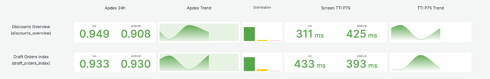


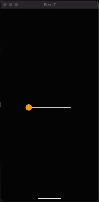


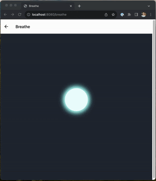


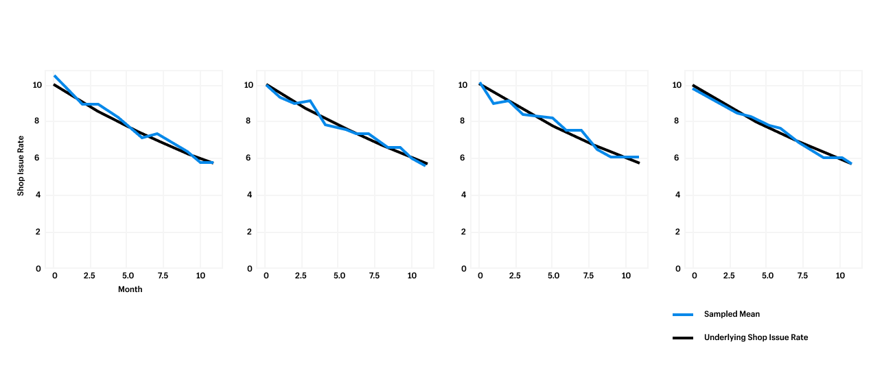


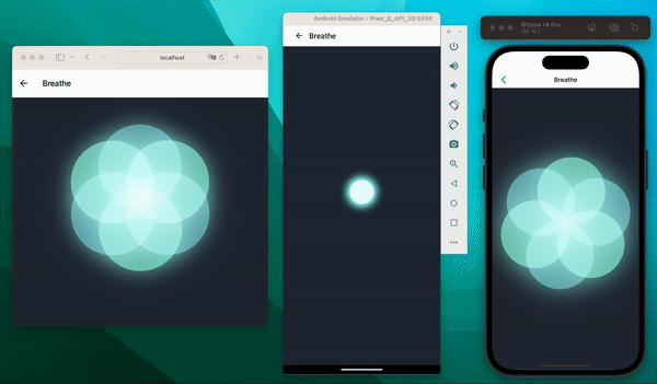


 Rails cache memcached fill percent versus time


